

Полная версия
Optical Engineering Science
4.4.2 Aberrations of a Thin Lens
We extend the treatment already outlined to analyse a thin lens. A thin lens can be considered as combination of two refractive surfaces, where the distance between the two surfaces is ignored. In practice, this is a reasonable assumption, provided the thickness is much less than the radii of the surfaces in question. Of course, the wavefront error produced by the two surfaces is simply the sum of the aberrations of the individual surfaces. A schematic for the analysis is shown in Figure 4.8.
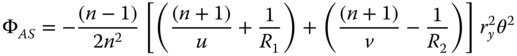
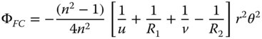
The wavefront error contribution for the first surface is very easy to compute; it is simply that set out in Eqs. (4.5a)–(4.5d). To compute the contribution for the second surface, one can analyse this using the same methodology as in Section 4.2, but exploiting natural symmetry. That is to say, one can analyse the second surface by rotating the whole surface about the y axis, such that z → −z and x → −x. In this event, for the second surface, R → −R2, u → v, θ → −θ. It is then simply a case of substituting these values into the formulae in Eqs. (4.5a)–(4.5d) and adding the wavefront error contribution of the first surface. The total wavefront error for the thin lens is then:
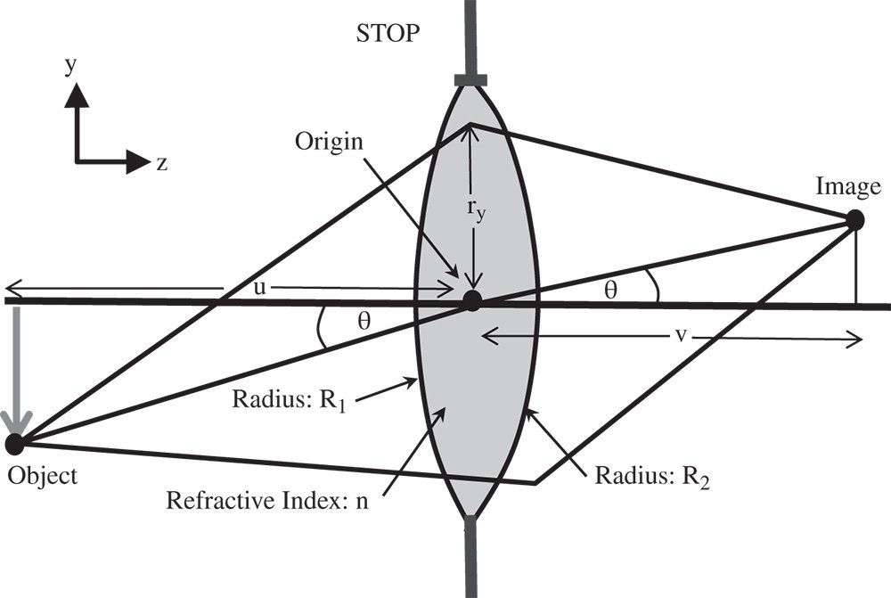
Figure 4.8 Aberration analysis for thin lens.


4.4.2.1 Conjugate Parameter and Lens Shape Parameter
In terms of gaining some insight into the behaviour of a thin lens, the formulae in Eqs. (4.25a)–(4.25d) are a little opaque. It would be somehow useful to express the aberrations of a thin lens directly in terms of its focusing power and some other parameters. The first of these other parameters is the so called conjugate parameter, t. The conjugate parameter is defined as below:
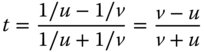
As we are dealing with a thin lens, we can use the thin lens formula to calculate the focal length, f, of the lens:
This, in turn, leads to expressions for u and v:
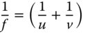
Figure 4.9 illustrates the conjugate parameter schematically. The infinite conjugate is represented by a conjugate parameter of ±1. If the conjugate parameter is +1, then the image is at infinity. Conversely, a conjugate parameter of −1 is associated with an object located at the infinite conjugate. In the symmetric scenario where object and image distances are identical, then the conjugate parameter is zero. As illustrated in Figure 4.9, where the conjugate parameter is greater than 1, then the object is real and the image is virtual. Finally, where the conjugate parameter is less than −1, then the object is virtual and the image is real.
Figure 4.9 Conjugate parameter.
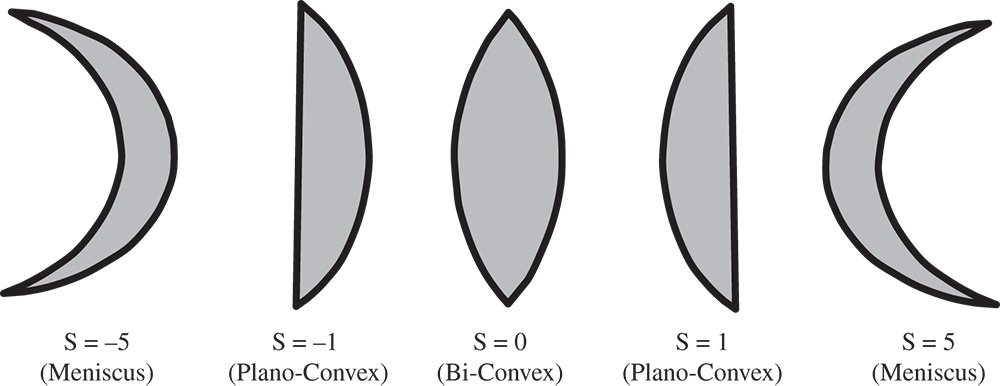
Figure 4.10 Coddington lens shape parameter.
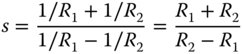
We have thus described object and image location in terms of a single parameter. By analogy, it is also useful to describe a lens in terms of its focal power and a single parameter that describes the shape of the lens. The lens, of course, is assumed to be defined by two spherical surfaces, with radii R1 and R2, defining the first and second surfaces respectively. The shape of a lens is defined by the so-called Coddington lens shape factor, s, which is defined as follows:
As before, the power of the lens may be expressed in terms of the lens radii:
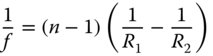
where n is the lens refractive index.
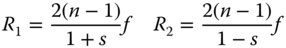
As with the conjugate parameter and the object and image distances, the two lens radii can be expressed in terms of the lens power and the shape factor, s.
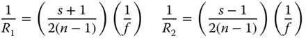
Figure 4.10 illustrates the lens shape parameter for a series of lenses with positive focal power. For a symmetric, bi-convex lens, the shape factor is zero. In the case of a plano-convex lens, the shape factor is 1 where the plane surface faces the image and is −1 where the plane surface faces the object. A shape factor of greater than 1 or less than −1 corresponds to a meniscus lens. Here, both radii have the same sense, i.e. they are either both positive or both negative. For a shape parameter of greater than 1, the surface with the greater curvature faces the object and for a shape parameter of less than −1, the surface with the greater curvature faces the image. Of course, this applies to lenses with positive power. For (diverging) lenses with negative power, then the sign of the shape factor is opposite to that described here.
4.4.2.2 General Formulae for Aberration of Thin Lenses
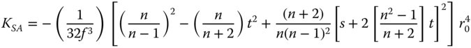
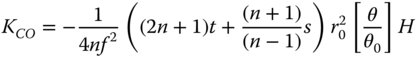
Having parameterised the object and image distances and the lens radii in terms of the conjugate parameter, shape parameter, and lens power, we can recast the expressions in Eqs. (4.25a)–(4.25d) in a more generic form. With a little algebraic manipulation, we obtain the following expressions for the Gauss-Seidel aberration of a lens with the stop at the lens surface:
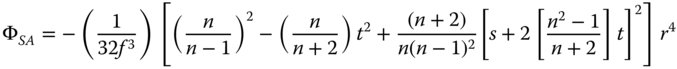
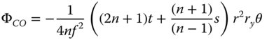
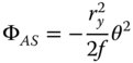
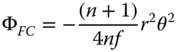
Again, casting all expressions in the form set out in Chapter 3, as for the expressions for the mirror we have
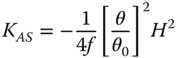
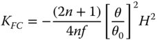
Once again, the Petzval curvature is simply given by subtracting twice the KAS term in Eq. (4.31c) from the field curvature term in Eq. (4.31d). This gives:
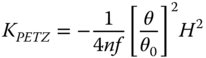
That is to say, a single lens will produce a Petzval surface whose radius of curvature is equal to the lens focal length multiplied by its refractive index. Once again, the Petzval sum may be invoked to give the Petzval curvature for a system of lenses:
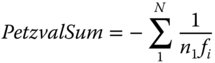
It is important here to re-iterate the fact that for a system of lenses, it is impossible to eliminate Petzval curvature where all lenses have positive focal lengths. For a system with positive focal power, i.e. with a positive effective focal length, there must be some elements with negative power if one wishes to ‘flatten the field’.
Before considering the aberration behaviour of simple lenses in a little more detail, it is worth reflecting on some attributes of the formulae in Eqs. (4.30a)–(4.30d). Both spherical aberration and coma are dependent upon the lens shape and conjugate parameters. In the case of spherical aberration there are second order terms present for both shape and conjugate parameters, whereas the behaviour for coma is linear. However, the important point to recognise is that the field curvature and astigmatism are independent of both lens shape and conjugate parameter and only depend upon the lens power. Once again, it must be emphasised that this analysis applies only to the situation where the stop is situated at the lens.
4.4.2.3 Aberration Behaviour of a Thin Lens at Infinite Conjugate
We will now look at a simple special case to apply to a thin lens with the stop at the lens. This is the common situation where a lens is being used to focus an object located at the infinite conjugate, such as a telescope objective or a lens focusing a parallel laser beam. From Eq. (4.26), the conjugate parameter, t, is equal to −1. Substituting t = −1 into Eq. (4.31a) gives the spherical aberration as:
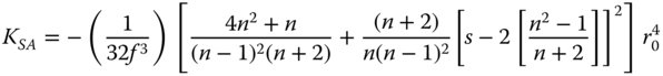
The important point to note about Eq. (4.34) is that the spherical aberration can never be equal to zero and that for a positive lens, KSA is always negative. This means that the longitudinal aberration for a positive lens is also negative and that, for all single lenses, more marginal rays are brought to a focus closer to the lens. Whilst Eq. (4.34) asserts that the spherical aberration in this case can never be zero, its magnitude can be minimised for a specific lens shape. Inspection of Eq. (4.34) reveals that this condition is met where:
This optimum shape factor corresponds to the so-called ‘best form singlet’ and is generally available from optical component suppliers, particularly with regard to applications in the focusing of laser beams. For a refractive index of 1.5, the optimum shape factor is around 0.7. This is close in shape to a plano-convex lens. However, it is important to emphasise, that optimum focusing is obtained where the more steeply curved surface is facing the infinite conjugate. Generally, also, where a plano-convex lens is used to focus a collimated beam, the curved surface should face the infinite conjugate. This behaviour is shown in Figure 4.11, which emphasises the quadratic dependence of spherical aberration on lens shape factor.
Coma for the infinite conjugate also depends upon the shape factor. However, in this instance, the dependence is linear. Once more, substituting t = −1 into Eq. (4.31b), we get:
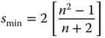
Unlike in the case for spherical aberration, there exists a shape factor for which the coma is zero. This is simply given by:
For a refractive index of 1.5, this minimum condition is met for a shape factor of 0.8. This is similar, but not quite the same as the optimum for spherical aberration. Again, the most curved surface should face the infinite conjugate. Overall behaviour is illustrated in Figure 4.12.
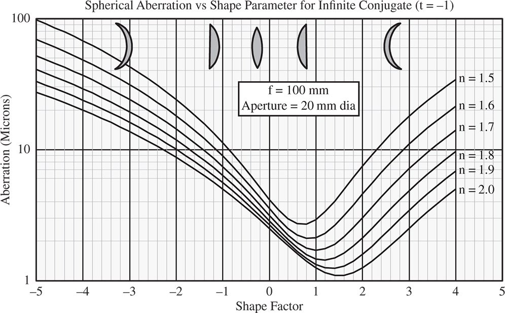
Figure 4.11 Spherical aberration vs. shape parameter for a thin lens.
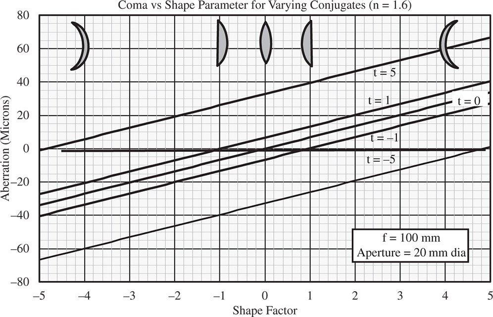
Figure 4.12 Coma vs lens shape for various conjugate parameters.
Once again, this specifically applies to the situation where the stop is at the lens surface. Of course, as stated previously, neither astigmatism nor field curvature are affected by shape or conjugate parameter.
Although it is impossible to reduce spherical aberration for a thin lens to zero at the infinite conjugate, it is possible for other conjugate values. In fact, the magnitude of the conjugate parameter must be greater than a certain specific value for this condition to be fulfilled. This magnitude is always greater than one for reasonable values of the refractive index and so either object or image must be virtual. It is easy to see from Eq. (4.31a) that this threshold value should be:
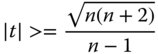
For n = 1.5, this threshold value is 4.58. That is to say for there to be a shape factor where the spherical aberration is reduced to zero, the conjugate parameter must either be less than −4.58 or greater than 4.58. Another point to note is that since spherical aberration exhibits a quadratic dependence on shape factor, where this condition is met, there are two values of the shape factor at which the spherical aberration is zero. This behaviour is set out in Figure 4.13 which shows spherical aberration as a function of shape factor for a number of difference conjugate parameters.
Worked Example 4.3 Best form Singlet
A thin lens is to be used to focus a Helium-Neon laser beam. The focal length of the lens is to be 20 mm and the lens is required to be ‘best form’ to minimise spherical aberration. The refractive index of the lens is 1.518 at the laser wavelength of 633 nm. Calculate the required shape factor and the radii of both lens surfaces. From Eq. (4.35) we have:
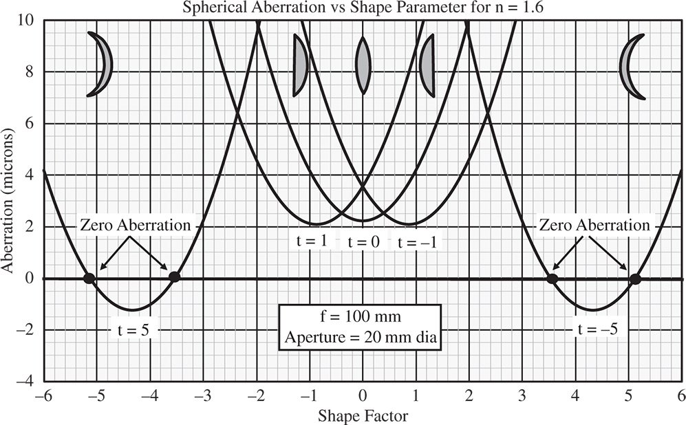
Figure 4.13 Spherical aberration vs shape factor for various conjugate parameter values.
The optimum shape factor is 0.742 and we can use this to calculate both radii given knowledge of the required focal length. Rearranging Eq. (4.29) we have:
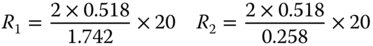
This gives:

It is the surface with the greatest curvature, i.e. R1, that should face the infinite conjugate (the parallel laser beam).
4.4.2.4 Aplanatic Points for a Thin Lens
Just as in the case of a single surface, it is possible to find a conjugate and lens shape pair that produce neither spherical aberration nor coma. For reasons outlined previously, it is not possible to eliminate astigmatism or field curvature for a lens of finite power. If the spherical aberration is to be zero, it must be clear that for the aplanatic condition to apply, then either the object or the image must be virtual. Equations (4.31a) and (4.31b) provide two conditions that uniquely determine the two parameters, s and t. Firstly, the requirement for coma to be zero clearly relates s and t in the following way:
Setting the spherical aberration to zero and substituting for t we have the following expression given entirely in terms of s:

and

Finally this gives the solution for s as:
Accordingly the solution for t is
Of course, since the equation for spherical aberration gives quadratic terms in s and t, it is not surprising that two solutions exist. Furthermore, it is important to recognise that the sign of t is the opposite to that of s. Referring to Figure 4.10, it is clear that the form of the lens is that of a meniscus. The two solutions for s correspond to a meniscus lens that has been inverted. Of course, the same applies to the conjugate parameter, so, in effect, the two solutions are identical, except the whole system has been inverted, swapping the object for image and vice-versa.
An aplanatic meniscus lens is an important building block in an optical design, in that it confers additional focusing power without incurring further spherical aberration or coma. This principle is illustrated in Figure 4.14 which shows a meniscus lens with positive focal power.
It is instructive, at this point to quantify the increase in system focal power provided by an aplanatic meniscus lens. Effectively, as illustrated in Figure 4.14, it increases the system numerical aperture in (minus) the ratio of the object and image distance. For the positive meniscus lens in Figure 4.14, the conjugate parameter is negative and equal to −(n + 1)/(n − 1). From Eq. (4.27) the ratio of the object and image distances is given by:
As previously set out, the increase in numerical aperture of an aplanatic meniscus lens is equal to minus the ratio of the object and image distances. Therefore, the aplanatic meniscus lens increases the system power by a factor equal to the refractive index of the lens. This principle is of practical consequence in many system designs. Of course, if we reverse the sense of Figure 4.14 and substitute the image for the object and vice versa, then the numerical aperture is effectively reduced by a factor of n.
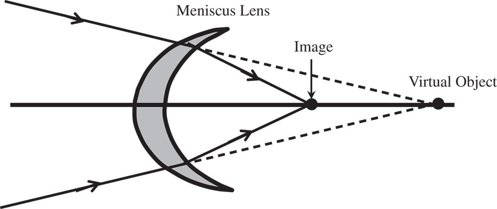
Figure 4.14 Aplanatic meniscus lens.
Worked Example 4.4 Microscope Objective – Hyperhemisphere Plus Meniscus Lens
We now wish to add some power to the microscope objective hyperhemisphere set out in Worked Example 4.1. We are to do so with an extra meniscus lens situated at the vertex of the hyperhemisphere with a negligible separation. As with the hyperhemisphere, the meniscus lens is in the aplanatic arrangement. The meniscus lens is made of the same material as the hyperhemisphere, that is with a refractive index of 1.6. All properties of the hyperhemisphere are as set out in Worked Example 4.1.
What are the radii of curvature of the meniscus lens and what is the location of the (virtual) image for the combined system? The system is as illustrated below.
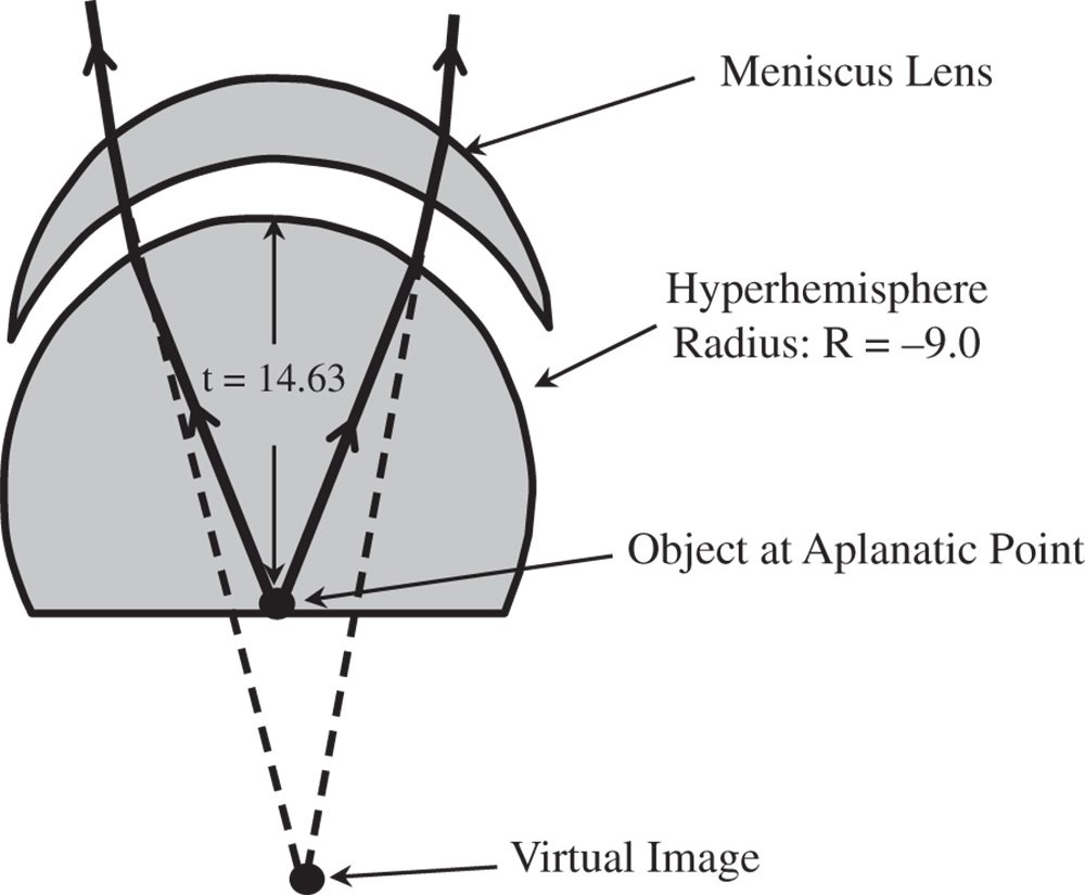
We know from Worked Example 4.1 that the original image distance produced by the hyperhemisphere is −23.4 mm. The object distance for the meniscus lens is thus 23.4 mm. From Eq. (4.39a) we have:
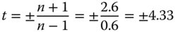
There remains the question of the choice of the sign for the conjugate parameter. If one refers to Figure 4.14, it is clear that the sense of the object and image location is reversed. In this case, therefore, the value of t is equal to +4.33 and the numerical aperture of the system is reduced by a factor of 1.6 (the refractive index). In that case, the image distance must be equal to minus 1.6 times the object distance. That is to say:

We can calculate the focal length of the lens from:
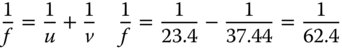
Therefore the focal length of the meniscus lens is 62.4 mm. If the conjugate parameter is +4.33, then the shape factor must be −(2n + 1), or −4.2 (note the sign). It is a simple matter to calculate the radii of the two surfaces from Eq. (4.29):
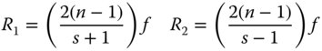
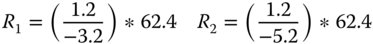
Finally, this gives R1 as −23.4 mm and R2 as −14.4 mm. The signs should be noted. This follows the convention that positive displacement follows the direction from object to image space.
If the microscope objective is ultimately to provide a collimated output – i.e. with the image at the infinite conjugate, the remainder of the optics must have a focal length of 37.44 mm (i.e. 23.4 × 1.6). This exercise illustrates the utility of relatively simple building blocks in more complex optical designs. This revised system has a focal length of 9 mm. However, the ‘remainder’ optics have a focal length of 37.4 mm, or only a quarter of the overall system power. Spherical aberration increases as the fourth power of the numerical aperture, so the ‘slower’ ‘remainder’ will intrinsically give rise to much less aberration and, as a consequence, much easier to design. The hyperhemisphere and meniscus lens combination confer much greater optical power to the system without any penalty in terms of spherical aberration and coma. Of course, in practice, the picture is complicated by chromatic aberration caused by variations in refractive properties of optical materials with wavelength. Nevertheless, the underlying principles outlined are very useful.
4.5 The Effect of Pupil Position on Element Aberration
In all previous analysis, it is assumed that the stop is located at the optical surface in question. This is a useful starting proposition. However, in practice, this is most usually not the case. With the stop located at a spherical surface, by definition, the chief ray will pass directly through the vertex of that surface. If, however, the surface is at some distance from the stop, then the chief ray will, in general, intersect the surface at some displacement from the surface vertex. This displacement is, in the first approximation, proportional to the field angle of the object in question. The general concept is illustrated in Figure 4.15.
Instead of the stop being located at the surface in question, the stop is displaced by a distance, s, from the surface. The chief ray, passing through the centre of the stop defines the field angle, θ. In addition, the pupil co-ordinates defined at the stop are denoted by rx and ry. However, if the stop were located at the optical surface, then the field angle would be θ′, as opposed to θ. In addition, the pupil co-ordinates would be given by rx′ and ry′. Computing the revised third order aberrations proceeds upon the following lines. All the previous analysis, e.g. as per Eqs. (4.31a)–(4.31d), has enabled us to express all aberrations as an OPD in terms of θ′, rx′, and ry′. It is clear that to calculate the aberrations for the new stop locations, one must do so in terms of the new parameters θ, rx, and ry. This is done by effecting a simple linear transformation between the two sets of parameters. Referring to Figure 4.15, it is easy to see:
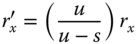
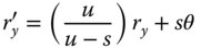
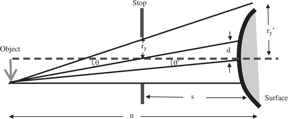
Figure 4.15 Impact of stop movement.

The effective size of the pupil at the optic is magnified by a quantity Mp and the pupil offset set out in Eq. (4.40b) is directly related to the eccentricity parameter, E, described in Chapter 2. Indeed, the product of the eccentricity parameter and the Lagrange invariant, H is simply equal to the ratio of the marginal and chief ray height at the pupil. That is to say: