Optical Engineering Science

Table 7.5 Luminous efficiencies of different sources.

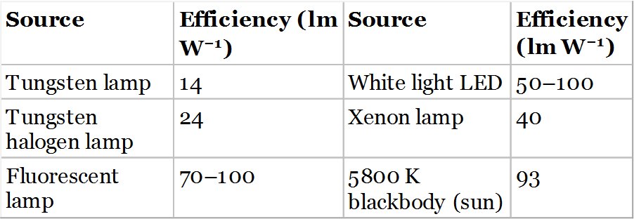
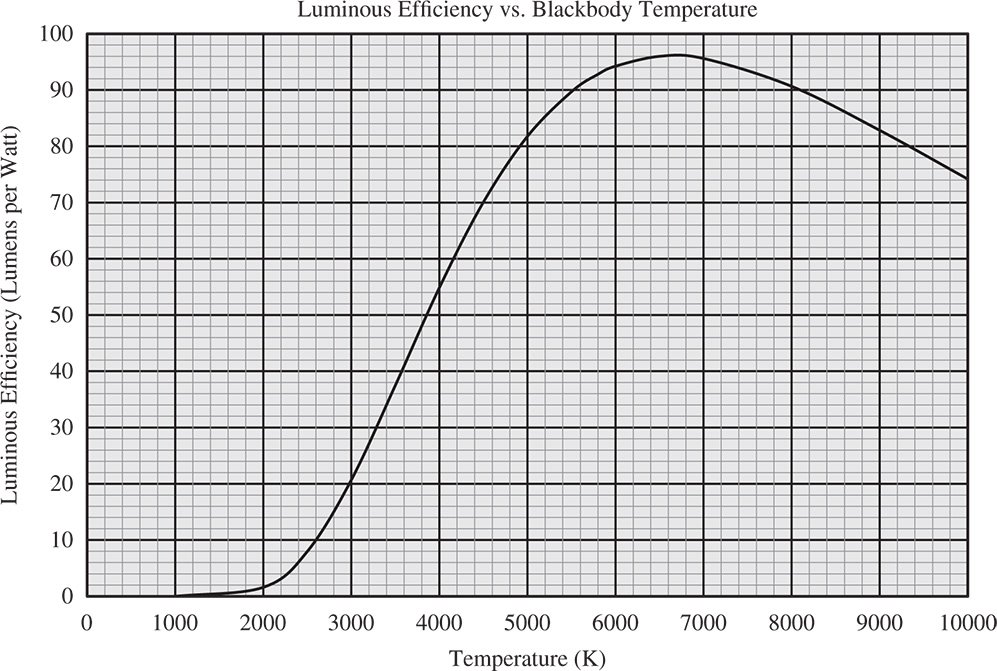
Figure 7.21 Luminous efficiency vs. blackbody temperature.

In fact, the luminous efficiency of a blackbody source may be calculated directly from the Planck distribution set out in Eq. (7.9) and the luminous efficiency function, V(λ). The plot is shown in Figure 7.21. The peak efficiency occurs around 6000 K and it is, of course, no coincidence that this is close to the solar blackbody temperature of 5800 K. Clearly, the human eye has been ‘designed’ to efficiently harvest light from its primary illumination source.

The brightness of different sources (to the human eye), or luminance, is expressed in candelas per square metre or nits. Representative values range from 80 cdm−2 for a typical cinema screen to 7 × 106 cdm−2 for the filament of an incandescent lamp and 1.6 × 109 cdm−2 for the solar disk. As for the luminous efficiency plot, the luminance of a blackbody source may be derived directly from the Planck distribution and the luminous efficiency curve, V(λ). This plot is shown in Figure 7.22.

7.7.4 Colour

7.7.4.1 Tristimulus Values

The preceding discussion has been wholly concerned with the level of illumination rather than (human) perception of the spectral distribution. This spectral distribution is described by the notion of colour, as perceived by humans. From the perspective of human vision, colour is discerned by the relative stimulation of three types of colour receptors (the cones). To model this process, the CIE, in 1931, proposed a set of colour matching functions, effectively mimicking the relative sensitivity of each type of sensor. The colour matching functions are represented as three separate curves, x(λ), y(λ), and z(λ), and operate, in principle, in a similar manner to the V(λ) curve for photopic efficiency. However, each curve is shifted with respect to the others. The form of these curves is illustrated in Figure 7.23.

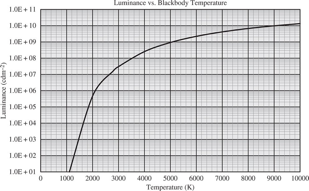
Figure 7.22 Luminance vs. blackbody temperature.

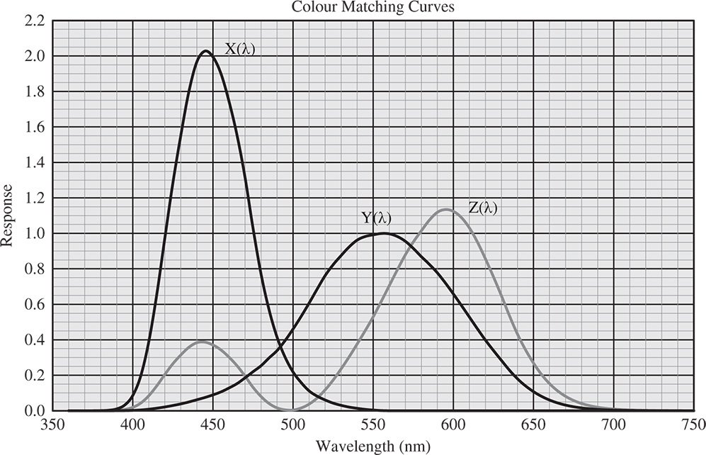
Figure 7.23 Colour matching curves.

It must be emphasised that the colour matching curves and the luminous efficiency curve are merely representative of human visual perception. These curves represent the fruits of sustained efforts to find a representative average of human perception. However, not surprisingly, there are considerable variations in spectral sensitivity between individuals.

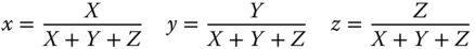
Quite significantly, the y(λ) curve follows that of the standard V(λ) curve. As for the basic photometric quantities, an input spectral radiance is transformed by integrating across the spectral range using the colour matching functions. However, instead of producing a single luminous flux value, three separate tristimulus values, X, Y, and Z are derived, as below.

(7.25)

From the preceding arguments, the Y tristimulus value is a measure of the luminance of the source. Normalisation of the tristimulus values provides a two dimensional description of colour.

(7.26)

Only the x and y ordinates are used in the standard CIE chromaticity diagram which provides a standardised quantification of the human perception of colour. The chromaticity diagram provides a plot in these two dimensions, with the third degree of freedom effectively corresponding to the luminous flux or intensity. Although it is perhaps obvious from the preceding discussion, this tripartite description of colour is purely an artefact of human vision and in no sense related to any property of light. Indeed, in recording any manifestly complex or subtle spectral distribution, the human eye can only, in effect, describe these by three independent parameters. It is clear that it is very possible for different spectral distributions to produce the same X, Y, Z stimulus values. This effect is known as metamerism. This highlights the limited spectral information that is provided by the three different sensor types. Indeed, two surface coatings (e.g. painted) can appear to be the same colour under one illumination (e.g. fluorescent) but different under another illumination source (e.g. tungsten) because of this effect.

7.7.4.2 RGB Colour

In many instances in describing colour we are interested in the effect of adding or blending colours. As a result of the three sensor types it is clear, in principle, that a linear combination of three different colours may be used to create a wide range colour sensations. The three colours themselves are described by a linear combination of the tristimulus values, X, Y, and Z and are known as primary colours. Definition of the suite of primary colours is arbitrary and established by virtue of convention. The guiding principle is that these three colours must be capable of being admixed to create as wide as possible a range of colours without recourse to negative coefficients in the linear combination. This range is referred to as a gamut. The original standard (1931 CIE) colour representation is the so-called RGB system (Red – Green – Blue) of primary colours using three standard monochromatic stimuli at 700 nm (R), 546.1 nm (G), and 435.8 nm (B). In this scheme, definition of the RGB primary colours from the tristimulus values is given by the following (X, Y, Z) vectorial representation:

(7.27)

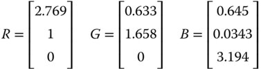
The inverse transformation between the two representations is effected by the following matrix:

(7.28)

Presentation of this RGB colour convention is intended for illustrative purposes only. This simple scheme has been largely superseded. In reality, there are a plethora of different primary colour conventions designed with specific applications, such computer screen rendition and so on, in mind. Some conventions take account of the non-linearity of the eye's response. That is to say, we abandon the linear convention hitherto prescribed. Other conventions ensure that uniform movements across colour space correspond to uniform changes in human perception of colour. These are called perceptually uniform colour spaces.

In principle, an equal admixture of primary colour components leads some form of standard white colouration or ‘white point’. The concept of whiteness as a chromatic descriptor is purely associated with the human perception of colour, rather than a fundamental property of a source. However, definition of whiteness, is convention dependent. Rather than defining a colour sensation by virtue of the admixture of RGB, it may also be defined by another three parameter set, HSL or hue, saturation, and luminosity. Hue is a measure of the undiluted colour, loosely corresponding to the equivalent monochromatic wavelength of stimulation. Saturation describes the purity of the colour, or the extent to which white must be admixed with a pure monochromatic colour to achieve the desired colour. The final degree of freedom is provided by luminosity which correlates to the brightness of the sensation, effectively the sum of the RGB components.

Colour difference, ΔE, is a measure of the absolute difference in colour between two different colours. It is generally expressed as the root sum of squares of the difference in each of the three colour ordinates and dependent upon the convention adopted. With this in mind, the concept of colour temperature describes the temperature of the blackbody radiator that most closely matches the colour of interest, i.e. with the smallest colour difference. This is particularly associated with the characterisation of light sources. Somewhat ironically, the term ‘cool’ describes a source with a bluer spectral distribution whereas a ‘warm’ light source refers to illumination with a larger red contribution. This is rather based on human perception and psychology; a ‘cool’, bluer blackbody source is, of course, hotter than a redder ‘warm’ source.

Much of the preceding discussion introduces the topic of colour with treatment of just one, antecedent, colour convention. As such, this provides a useful description of the basic underlying principles. However, the topic in itself is much too broad to provide any comprehensive treatment here and the reader is referred to specialist texts for further study. Some guidance is provided in the short bibliography and the end of the chapter.

7.7.5 Astronomical Photometry

Astronomical photometry is concerned with the measurement of the magnitude of electromagnetic flux from stellar objects, stars galaxies, and so on. For modern observations, these measurements are almost exclusively dependent upon semi-conductor detectors. For a given stellar object, the ideal measurement might involve the high resolution capture of its spectral irradiance at the earth across a wide range of wavelengths. That is to say, a detailed spectrum of each object should be obtained that can be related to absolute spectral irradiance. However, as stellar objects of interest are almost invariably faint, the amount of flux that is captured in any given wavelength band is necessarily very small. For the majority of measurements, therefore, this approach is impractical. A more practical solution is to use a number of spectrally filtered detectors to monitor flux from the star (via a telescope). Each filter has a relatively broad passband, e.g. 100 nm and centred on some specific wavelength, e.g. 555 nm. Using a small number of these filtered detectors across the ultraviolet, visible, and infrared spectral ranges, provides what amounts to low resolution spectral information for the source. However, since interpretation of the spectral quality of a stellar object is based on a limited number (e.g. 3) of spectrally filtered measurements, there is a clear correlation with visual photometry.