

Полная версия
Optical Engineering Science
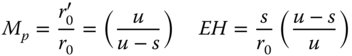
In this case, r0 refers to the pupil radius at the stop and r0′ to the effective pupil radius at the surface in question. As a consequence, we can re-cast all three equations in a more convenient form.
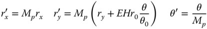
The angle, θ0 is representative of the maximum system field angle and helps to define the eccentricity parameter and the Lagrange invariant. We already know the OPD when cast in terms of rx′, ry′, and θ, as this is as per the analysis for the case where the stop is at the optic itself. That is to say, the expression for the OPD is as given in Eqs. and these aberrations defined in terms of KSA′, KCO′, KAS′, KFC′, and KDI′. Therefore, the total OPD attributable to the five Gauss-Seidel aberrations is given by:

To determine the aberrations as expressed by the pupil co-ordinates for the new stop location, it is a simple matter of substituting Eq. (4.42) into Eq. (4.43). This results in the so-called stop shift equations:

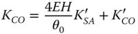
What this set of equations reveals is that there exists a ‘hierarchy’ of aberrations. Spherical aberration may be transmuted into coma, astigmatism, field curvature, and distortion by shifting the stop position. Similarly, coma may be transformed into astigmatism, field curvature, and distortion and both astigmatism and field curvature may produce distortion. However, coma can never produce spherical aberration and neither astigmatism nor field curvature is capable of generating spherical aberration or coma. Equation (4.44e) reveals, for the first time, that it is possible to generate distortion by shifting the stop. Our previous idealised analysis clearly suggested that distortion is not produced where the lens or optical surface is located at the stop.
Another important conclusion relating to Eqs. (4.44a)–(4.44e) is the impact of stop shift on the astigmatism and field curvature. Inspection of Eqs. (4.44c) and (4.44d) reveals that the change in field curvature produced by stop shift is precisely double that of the change in astigmatism in all cases. Therefore, the Petzval curvature, which is given by KFC−2KAS remains unchanged by stop shift. This further serves to demonstrate the fact that the Petzval curvature is a fundamental system attribute and is unaffected by changes in stop location and, indeed component location. Petzval curvature only depends upon the system power. Thus, it is important to recognise that the quantity KFC−2KAS is preserved in any manipulation of existing components within a system. If we express the Petzval curvature in terms of the tangential and sagittal curvature we find:

Since KPetz is not changed by any manipulation of component or stop positions, Eq. (4.45) implies that any change in the sagittal curvature is accompanied by a change three times as large in the tangential curvature. This is an important conclusion.
For small shifts in the position of the stop, the eccentricity parameter is proportional to that shift. Based on this and examining Eqs. (4.44a)–(4.44e), one can come to some general conclusions. For a system with pre-existing spherical aberration, additional coma will be produced in linear proportion to the stop shift. Similarly, the same spherical aberration will produce astigmatism and field curvature proportional to the square of the stop shift. The amount of distortion produced by pre-existing spherical aberration is proportional to the cube of the displacement. Naturally, for pre-existing coma, the additional astigmatism and field curvature produced is in proportion to the shift in the stop position. Additional distortion is produced according to the square of the stop shift. Finally, with pre-existing astigmatism and field curvature, only additional distortion may be produced in direct proportion to the stop shift.
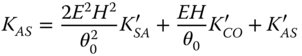
As an example, a simple scenario is illustrated in Figure 4.16. This shows a symmetric system with a biconvex lens used to image an object in the 2f – 2f configuration. That is to say, the conjugate parameter is zero. In this situation, the coma may be expected, by virtue of symmetry, to be zero. For a simple lens, the distortion is also zero. The spherical aberration is, of course, non-zero, as are both the astigmatism and field curvature.
Using basic modelling software, it is possible to analyse the impact of small stop shifts on system aberration. The results are shown in Figure 4.17.
Clearly, according to Figure 4.17, the spherical aberration remains unchanged as predicted by Eq. (4.44a). For small shifts, the amount of coma produced is in proportion to the shift. Since there is no coma initially, the only aberration that can influence the astigmatism and field curvature is the pre-existing spherical aberration. As indicated in Eqs. (4.44c) and (4.44d), there should be a quadratic dependence of the astigmatism and field curvature on stop position. This is indeed borne out by the analysis in Figure 4.17. Similarly, the distortion shows a linear trend with stop position, mainly influenced by the initial astigmatism and field curvature that is present.
Although, in practice, these stop shift equations may not find direct use currently in optimising real designs, the underlying principles embodied are, nonetheless, important. Manipulation of the stop position is a key part in the optimisation of complex optical systems and, in particular, multi-element camera lenses. In these complex systems, the pupil is often situated between groups of lenses. In this case, the designer needs to be aware also of the potential for vignetting, should individual lens elements be incorrectly sized.
Figure 4.16 Simple symmetric lens system with stop shift.
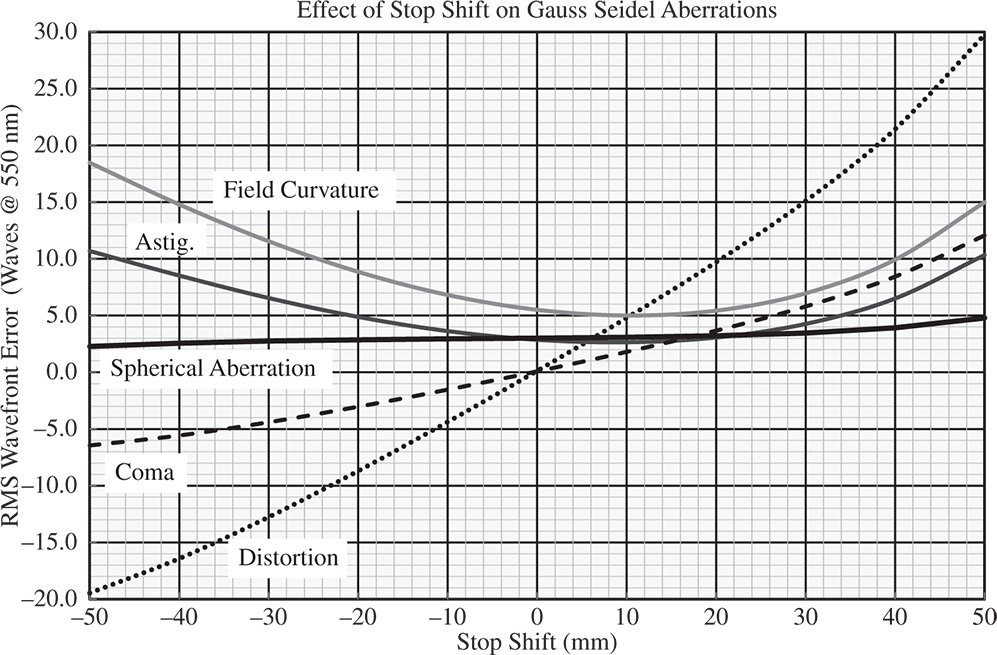
Figure 4.17 Impact of stop shift for simple symmetric lens system.
The stop shift equations provide a general insight into the impact of stop position on aberration. Most significant is the hierarchy of aberrations. For example, no fundamental manipulation of spherical aberration may be accomplished by the manipulation of stop position. Otherwise, there some special circumstances it would be useful for the reader to be aware of. For example, in the case of a spherical mirror, with the object or image lying at the infinite conjugate, the placement of the stop at the mirror's centre of curvature altogether removes its contribution to coma and astigmatism; the reader may care to verify this.
4.6 Abbe Sine Condition
Long before the advent of powerful computer ray tracing models, there was a powerful incentive to develop simple rules of thumb to guide the optical design process. This was particularly true for the complex task of ameliorating system aberrations. Working in the nineteenth century, Ernst Abbe set out the Abbe sine condition, which directly relates the object and image space numerical apertures for a ‘perfect’, unaberrated system. Essentially, the Abbe sine condition articulates a specific requirement for a system to be free of spherical aberration and coma, i.e. aplanatic. The Abbe sine condition is expressed for an infinitesimal object and image height and its justification is illustrated in Figure 4.18.
In the representation in Figure 4.18 we trace a ray from the object to a point, P, located on a reference sphere whose centre lies on axis at the axial position of the object and whose vertex lies at the entrance pupil. At the same time, we also trace a marginal ray from the object location to the entrance pupil. The conjugate point to P, designated, P′, is located nominally at the exit pupil and on a sphere whose centre lies at the paraxial image location. For there to be perfect imaging, then the OPD associated with the passage of the marginal ray must be zero. Furthermore, the OPD of the ray from object to image must also be zero. It is also further assumed that the relative OPD of the object to image ray when compared to the marginal ray is zero on passage from points P to P′. This assumption is justified for an infinitesimal object height. Therefore, it is possible to compute the total object to image OPD by simply summing the path differences relative to the marginal ray between the object and point P and between the image and point P′. For there to be perfect imaging this difference must, of course be zero.
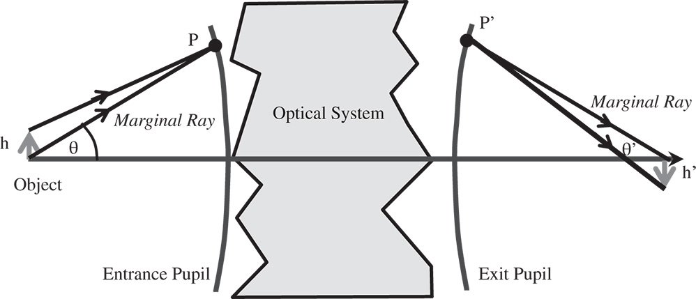
Figure 4.18 Abbe sine condition.

n is the refractive index in object space and n′ is the refractive index in image space.
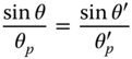
Equation 4.46 is one formulation of the Abbe sine condition which, nominally, applies for all values of θ and θ′, including paraxial angles. If we represent the relevant paraxial angles in object and image space as θp and θp' then the Abbe sine condition may be rewritten as:
One specific scenario occurs where the object or image lies at the infinite conjugate. For example, one might imagine an object located on axis at the first focal point. In this case, the height of any ray within the collimated beam in image space is directly proportional to the numerical aperture associated with the input ray.
Figure 4.19 illustrates the application of the Abbe sine condition for a specific example. As highlighted previously, the sine condition effectively seeks out the aplanatic condition in an optical system. In this example, a meniscus lens is to be designed to fulfil the aplanatic condition. However, its conjugate parameter is adjusted around the ideal value and the spherical aberration and coma plotted as a function of the conjugate parameter. In addition, the departure from the Abbe sine condition is also plotted in the same way. All data is derived from detailed ray tracing and values thus derived are presented as relative values to fit reasonably into the graphical presentation. It is clear that elimination of spherical aberration and coma corresponds closely to the fulfilment of the Abbe sine condition.
The form of the Abbe sine condition set out in Eq. (4.46) is interesting. It may be compared directly to the Helmholtz equation which has a similar form. However, instead of a relationship based on the sine of the angle, the Helmholtz equation is defined by a relationship based on the tangent of the angle:

It is quite apparent that the two equations present something of a contradiction. The Helmholtz equation sets the condition for perfect imaging in an ideal system for all pairs of conjugates. However, the Abbe sine condition relates to aberration free imaging for a specific conjugate pair. This presents us with an important conclusion. It is clear that aberration free imaging for a specific conjugate (Abbe) fundamentally denies the possibility for perfect imaging across all conjugates (Helmholtz). Therefore, an optical system can only be designed to deliver aberration free imaging for one specific conjugate pair.
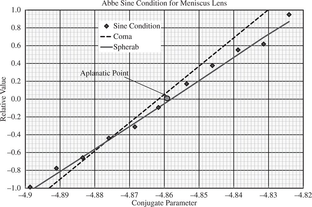
Figure 4.19 Fulfilment of Abbe sine condition for aplanatic meniscus lens.
4.7 Chromatic Aberration
4.7.1 Chromatic Aberration and Optical Materials
Hitherto, we have only considered the classical monochromatic aberrations. At this point, we must introduce the phenomenon of chromatic aberration where imperfections in the imaging of an optical system are produced by significant variation in optical properties with wavelength. All optical materials are dispersive to some degree. That is to say, their refractive indices vary with wavelength. As a consequence, all first order properties of an optical system, such as the location of the cardinal points, vary with wavelength. Most particularly, the paraxial focal position of an optical system with dispersive components will vary with wavelength, as will its effective focal length. Therefore, for a given axial position in image space, only one wavelength can be in focus at any one time.
Dispersion is a property of transmissive optical materials, i.e. glasses. On the other hand, mirrors show no chromatic variation and their incorporation is favoured in systems where chromatic variation is particularly unwelcome. Such a system, where the optical properties do not vary with wavelength, is said to be achromatic. As argued previously, a mirror behaves as an optical material with a refractive index of minus one, a value that is, of course, independent of wavelength. In general, the tendency in most optical materials is for the refractive index to decrease with increasing wavelength. This behaviour is known as normal dispersion. In certain very specific situations, for certain materials at particular wavelengths, the refractive index actually decreases with wavelength; this phenomenon is known as anomalous dispersion.
Although dispersion is an issue of concern covering all wavelengths of interest from the ultraviolet to the infrared, for obvious reasons, historically, there has been particular focus on this issue within the visible portion of the spectrum. Across the visible spectrum, for typical glass materials, the refractive index variation might amount to 0.7–2.5%. This variation in the dispersive properties of different materials is significant, as it affords a means to reduce the impact of chromatic aberration as will be seen shortly. Figure 4.20 shows a typical dispersive plot, for the glass material, SCHOTT BK7®.
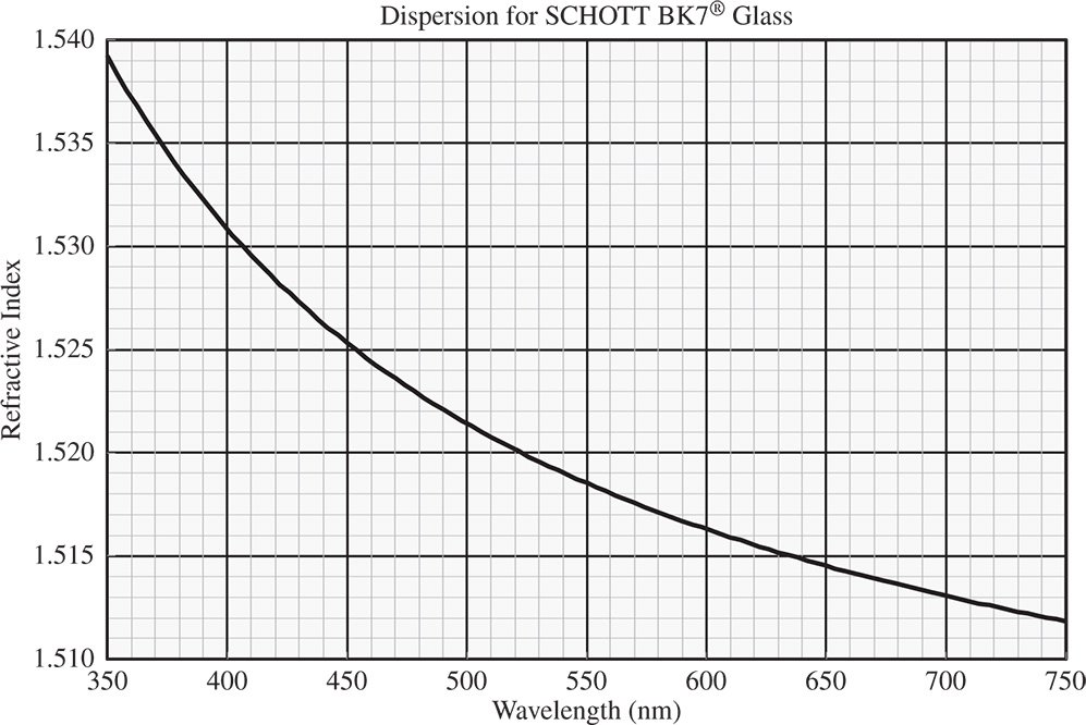
Figure 4.20 Refractive index variation with wavelength for SCHOTT BK7 glass material.
Because of the historical importance of the visible spectrum, glass materials are typically characterised by their refractive properties across this portion of the spectrum. More specifically, glasses are catalogued in terms of their refractive indices at three wavelengths, nominally ‘blue’, ‘yellow’, and ‘red’. In practice, there are a number of different conventions for choosing these reference wavelengths, but the most commonly applied uses two hydrogen spectral lines – the ‘Balmer-beta’ line at 486.1 nm and the ‘Balmer-alpha’ line at 656.3, plus the sodium ‘D’ line at 589.3 nm. The refractive indices at these three standard wavelengths are symbolised as nF, nC, and nD respectively. At this point, we introduce the Abbe number, VD, which expresses a glass's dispersion by the ratio of its optical power to its dispersion:
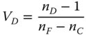
The numerator in Eq. (4.48) represents the effective optical or focusing power at the ‘yellow’ wavelength, whereas the denominator describes the dispersion of the glass as the difference between the ‘blue’ and the ‘red’ indices. It is important to recognise that the higher the Abbe number, then the less dispersive the glass, and vice versa. Abbe numbers vary, typically between about 20 and 80. Broadly speaking, these numbers express the ratio of the glass's focusing power to its dispersion. Hence, for a material with an Abbe number of 20, the focal length of a lens made from this material will differ by approximately 5% (1/20) between 486.1 and 656.3 nm.
4.7.2 Impact of Chromatic Aberration
The most obvious effect of chromatic aberration is that light is broad to a different focus for different wavelengths. This effect is known as longitudinal chromatic aberration and is illustrated in Figure 4.21.
As can be seen from Figure 4.21, light at the shorter, ‘blue’ wavelengths are focused closer to the lens, leading to an axial (longitudinal) shift in the paraxial focus for the different wavelengths. In summary, longitudinal chromatic aberration is associated with a shift in the paraxial focal position as a function of wavelength. Thus the effect of longitudinal chromatic aberration is to produce a blur spot or transverse aberration whose magnitude is directly proportional to the aperture size, but is independent of field angle. However, there are situations where, to all intents and purposes, all wavelengths share the same paraxial focal position, but the principal points are not co-located. That is to say, whilst all wavelengths are focused at a common point, the effective focal length corresponding to each wavelength is not identical. This scenario is illustrated in Figure 4.22.
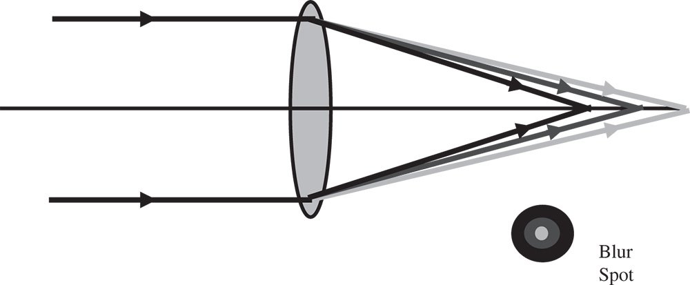
Figure 4.21 Longitudinal chromatic aberration.
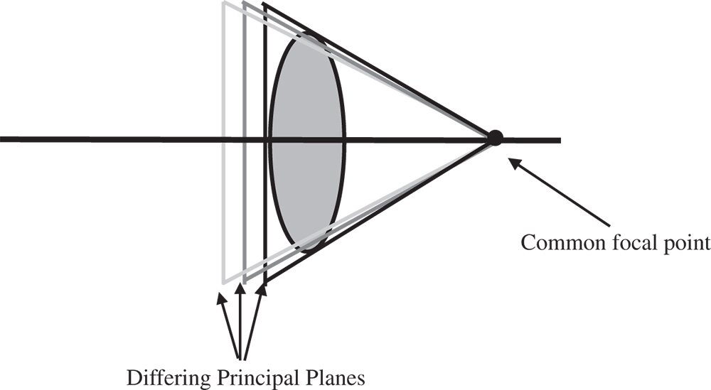
Figure 4.22 Transverse chromatic aberration.
The effect illustrated is known as transverse chromatic aberration or lateral colour. Whilst no distinct blurring is produced by this effect, the fact that different wavelengths have different focal lengths inevitably means that system magnification varies with wavelength. As a result, the final image size or height of a common object depends upon the wavelength. This produces distinct coloured fringing around an object and the size of the effect is proportional to the field angle, but independent of aperture size.
Hitherto, we have cast the effects of chromatic aberration in terms of transverse aberration. However, to understand the effect on the same basis as the Gauss-Seidel aberrations, it is useful to express chromatic aberration in terms of the OPD. When applied to a single lens, longitudinal chromatic aberration simply produces defocus that is equal to the focal length divided by the Abbe number. Therefore, the longitudinal chromatic aberration is given by:
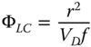
f is the focal length of the lens and r the pupil position.
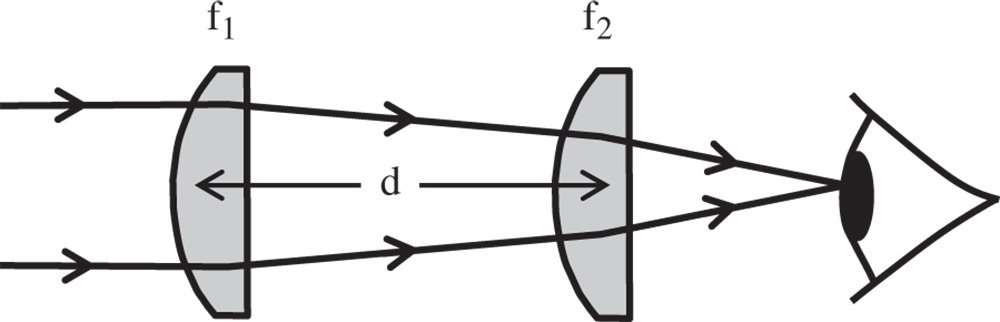
Figure 4.23 Huygens eyepiece.
Similarly, the transverse chromatic aberration can be expressed as an OPD:
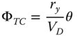
Examining Eqs. (4.49a) and (4.49b) reveals that the ratio of transverse to longitudinal aberration is given by the ratio of the field angle to the numerical aperture. In practice, for optical elements, such as microscope and telescope objectives, the field angle is very much smaller than the numerical aperture and thus longitudinal chromatic aberration may be expected to predominate. For eyepieces, the opposite is often the case, so the imperative here is to correct lateral chromatic aberration.
Worked Example 4.5 Lateral Chromatic Aberration and the Huygens Eyepiece
A practical example of the correction of lateral chromatic aberration is in the Huygens eyepiece. This very simple, early, eyepiece uses two plano-convex lenses separated by a distance equivalent to half the sum of their focal lengths. This is illustrated in Figure 4.23.

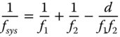
Since we are determining the impact of lateral chromatic aberration, we are only interested in the effective focal length of the system comprising the two lenses. Using simple matrix analysis as described in Chapter 1, the system focal length is given by:
If we assume that both lenses are made of the same material, then their focal power will change as a function of wavelength by a common proportion, α. In that case, the system focal power at the new wavelength would be given by:
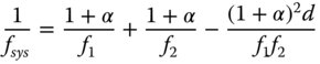
For small values of α, we can ignore terms of second order in α, so the change in system power may be approximated by:
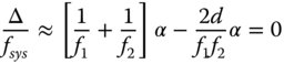
The change in system power should be zero and this condition unambiguously sets the lens separation, d, for no lateral chromatic aberration:

If this condition is fulfilled, then the Huygens eyepiece will have no transverse chromatic aberration. However, it must be emphasised that this condition does not provide immunity from longitudinal chromatic aberration.
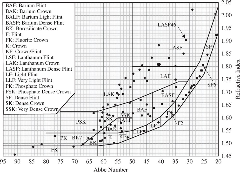
Figure 4.24 Abbe diagram.
4.7.3 The Abbe Diagram for Glass Materials
For visible applications, the Abbe number for a glass is of equal practical importance as the refractive index itself. The Abbe diagram is a simple graphic tool that captures the basic refractive properties of a wide range of optical glasses. It comprises a simple 2D map with the horizontal axis corresponding to the Abbe number and the vertical axis to the glass index. A representative diagram is shown in Figure 4.24.
By referring to this diagram, the optical designer can make appropriate choices for specific applications in the visible. In particular, it helps select combinations of glasses leading to a substantially achromatic design. One special and key application is the achromatic doublet. This lens is composed of two elements, one positive and one negative. The positive lens is a high power (short focal length) element with low dispersion and the negative lens is a low power element with high dispersion. Materials are chosen in such a way that the net dispersion of the two elements cancel, but the powers do not. This will be considered in more detail in the next section.
The different zones highlighted in the Abbe diagram replicated in Figure 4.24 refer to the elemental composition of the glass. For example, ‘Ba’ refers to the presence of barium and ‘La’ to the presence of lanthanum. Originally, many of the dense, high index glasses used to contain lead, but these are being phased out due to environmental concerns. The Abbe diagram reveals a distinct geometrical profile with a tendency for high dispersion to correlate strongly with refractive index. In fact, it is the presence of absorption features within the glass (at very much shorter wavelengths) that give rise to the phenomenon of refraction and these features also contribute to dispersion.
4.7.4 The Achromatic Doublet
As introduced previously, the achromatic doublet is an extremely important building block in a transmissive (non-mirror) optical design. The function of an achromatic doublet is illustrated in Figure 4.25.