

Полная версия
Optical Engineering Science
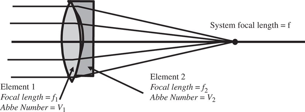
Figure 4.25 The achromatic doublet.
The first element, often (on account of its shape) referred to as the ‘crown element’, is a high power positive lens with low dispersion. The second element is a low power negative lens with high dispersion. The focal lengths of the two elements are f1 and f2 respectively and their Abbe numbers V1 and V2. Since the intention is that the dispersions of the two elements should entirely cancel, this condition constrains the relative power of the two elements. Individually, the dispersion as measured by the difference in optical power between the red and blue wavelengths is proportional to the reciprocal of the focal power and the Abbe number for each element. Therefore:
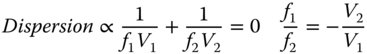
From Eq. (4.51), it is clear that the ratio of the two focal lengths should be minus the inverse of the ratio of their respective Abbe numbers. In other words, the ratio of their powers should be minus the ratio of their Abbe numbers. The power of the system comprising the two lenses is, in the thin lens approximation, simply equal to the sum of their individual powers. Therefore, it is possible to calculate these individual focal lengths, f1 and f2, in terms of the desired system focal length of f:

Thus, the two focal lengths are simply given by:
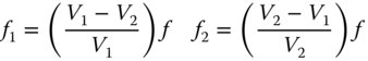
In the thin lens approximation, therefore, light will be focused at the same point for the red and blue wavelengths. Consequentially, in this approximation, this system will be free from both longitudinal and transverse chromatic aberration. The simplicity of this approach may be illustrated in a straightforward worked example.
Worked Example 4.6 Simple Achromatic Doublet
We wish to construct and achromatic doublet with a focal length of 200 mm. The two glasses to be used are: SCHOTT N-BK7 for the positive crown lens and SCHOTT SF2 for the negative lens. Both these glasses feature on the Abbe diagram in Figure 4.24 and the Abbe number for these glasses are 64.17 and 33.85 respectively. The individual focal lengths may be calculated using Eq. (4.52):
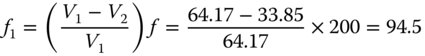
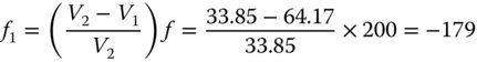
Therefore, the focal length of the first ‘crown lens’ should be 94.5 mm and the focal length of the second diverging lens should be −179 mm.
Thus far, the analysis design of an achromatic doublet has been fairly elementary. In the previous worked example, we have constrained the focal lengths of the two lens elements to specific values. However, we are still free to choose the shape of each lens. That is to say, there are two further independent variables that can be adjusted. Achromatic doublets can either be cemented or air spaced. In the case of the cemented doublet, as presented in Figure 4.25, the second surface of the first lens must have the same radius as the first surface of the second lens. This provides an additional constraint; thus, for the cemented doublet, there is only one additional free variable to adjust. However, introduction of an air space between the two lenses removes this constraint and gives the designer an extra degree of freedom to play with. That said, the cemented doublet does offer greater robustness and reliability with respect to changes in alignment and finds very wide application as a standard optical component.
As a ‘stock component’ achromatic doublets are designed, generally, for the infinite conjugate. For cemented doublets, with the single additional degree of design freedom, these components are optimised to have zero spherical aberration at the central wavelength. This is an extremely important consideration, for not only are these doublets free of chromatic aberration, but they are also well optimised for other aberrations. Commercial doublets are thus extremely powerful optical components.
4.7.5 Optimisation of an Achromatic Doublet (Infinite Conjugate)
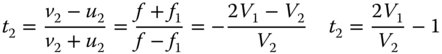
An air spaced achromatic doublet may be optimised to eliminate both spherical aberration and coma. The fundamental power of the wavefront approach in describing third order aberration is reflected in the ability to calculate the total system aberration as the sum of the aberration of the two lenses. In the thin lens approximation, we may simply use Eqs. (4.30a) and (4.30b) to express the spherical aberration and coma contribution for each lens element. We simply ascribe a variable shape parameter, s1 and s2 to each of the two lenses. The two conjugate parameters are fixed. In the particular case of a doublet designed for the infinite conjugate, the conjugate parameter for the first lens, t1, is −1. In the case of the second lens, the conjugate parameter, t2, is determined by the relative focal lengths of the two lenses and thus fixed by the ratio of the two Abbe numbers and, from Eq. (4.52), we get:
Without going through the algebra in detail, it is clear that having determined both t1 and t2, Eqs. (4.30a) and (4.30b) give us two expressions solely in terms of s1 and s2. These expressions for the spherical aberration and coma must be set to zero and can be solved for both s1 and s2. The important point to note about this procedure is that because Eq. 4.30a contains terms that are quadratic in shape factor, this is also reflected in the final solution. Therefore, in general, we might expect to find two solutions to the equation and this, in general, is true.
Worked Example 4.7 Detailed Design of 200 mm Focal Length Achromatic Doublet
At this point we illustrate the design of an air spaced achromat by looking more closely at the previous example where we analysed a 200 mm achromat design. We are to design an achromat with a focal length of 200 mm working at the infinite conjugate, using SCHOTT N-BK7 and SCHOTT SF2 as the two glasses, with the less dispersive N-BK7 used as the positive ‘crown’ element. Again, the Abbe numbers for these glasses are 64.17 and 33.85 respectively and the nd values (refractive index at 589.6 nm) 1.5168 and 1.647 69. From the previous example, we know that focal lengths of the two lenses are:

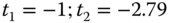
The two conjugate parameters are straightforward to determine. The first conjugate parameter, t1, is naturally −1. Eq. (4.53) can be used to determine the second conjugate parameter, t2. This gives:
We now substitute the conjugate parameter values together with the refractive index values (ND) into Eq. (4.30a). We sum the contributions of the two lenses giving the total spherical aberration which we set to zero. Calculating all coefficients we get a quadratic equation in terms of the two shape factors, s1 and s2.

We now repeat the same process for Eq. (4.30b), setting the total system coma to zero. This time we get a linear equation involving s1 and s2.

Substituting Eq. (4.55) into Eq. (4.54) gives the desired quadratic equation:
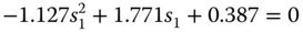
There are, of course, two sets of solutions to Eq. (4.56), with the following values:
Solution 1: s1 = −0.194; s2 = 1.823
Solution 2: s1 = 3.198; s2 = 2.929
There now remains the question as to which of these two solutions to select. Using Eq. (4.29) to calculate the individual radii of curvature from the lens shapes and focal length we get:
Solution 1: R1 = 121.25 mm; R2 = −81.78 mm; R3−81.29 mm; R4 = −281.88 mm
Solution 2: R1 = 23.26 mm; R2 = 44.43 mm; R3−58.91 mm; R4 = −119.68 mm
The radii R1 and R2 refer to the first and second surfaces of lens 1 and R3 and R4 to the first and second surfaces of lens 2. It is clear that the first solution contains less steeply curved surfaces and is likely to be the better solution, particularly for relatively large apertures. In the case of the second solution, whilst the solution to the third order equations eliminates third order spherical aberration and coma, higher order aberrations are likely to be enhanced.
The first solution to this problem comes under the generic label of the Fraunhofer doublet, whereas the second is referred to as a Gauss doublet. It should be noted that for the Fraunhofer solution, R2 and R3 are almost identical. This means that should we constrain the two surfaces to have the same curvature (in the case of a cemented doublet) and just optimise for spherical aberration, then the solution will be close to that of the ideal aplanatic lens. To do this, we would simply use Eq. 4.29, forcing R2 and R3 to be equal and to replace Eq. 4.55 constraining the total coma, providing an alternative relation between s1 and s2. However, the fact that the cemented doublet is close to fulfilling the zero spherical aberration and coma condition further illustrates the usefulness of this simple component.
The analysis presented applies only strictly in the thin lens approximation. In practice, optimisation of a doublet such as presented in the previous example would be accomplished with the aid of ray tracing software. However, the insights gained by this exercise are particularly important. For instance, in carrying out a computer-based optimisation, it is critically important to understand that two solutions exist. Furthermore, in setting up a computer-based optimisation, an exercise, such as this, provides a useful ‘starting point’.
4.7.6 Secondary Colour
The previous analysis of the achromatic doublet provides a means of ameliorating the impact of glass dispersion and to provide correction at two wavelengths. In the case of the standard visible achromat, correction is provided at the F and C wavelengths, the two hydrogen lines at 486.1 and 656.3 nm. Unfortunately, however, this does not guarantee correction at other, intermediate wavelengths. If one views dispersion of optical materials as a ‘small signal’ problem, and that any difference in refractive index is small across the region of interest, then correction of the chromatic focal shift with a doublet may be regarded as a ‘linear process’. That is to say we might approximate the dispersion of an optical material by some pseudo-linear function of wavelength, ignoring higher order terms. However, by ignoring these higher order terms, some residual chromatic aberration remains. This effect is referred to as secondary colour. The effect is illustrated schematically in Figure 4.26 which shows the shift in focus as a function of wavelength.
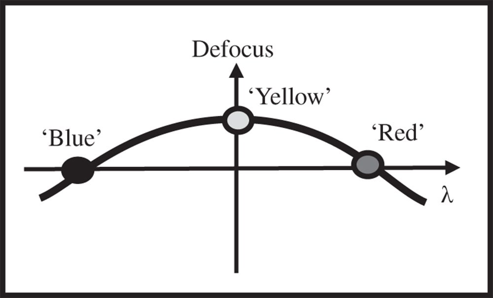
Figure 4.26 Secondary colour.
Figure 4.26 clearly shows the effect as a quadratic dependence in focal shift with wavelength, with the ‘red’ and ‘blue’ wavelengths in focus, but the central wavelength with significant defocus. In line with the notion that we are seeking to quantify a quadratic effect, we can define the partial dispersion coefficient, P, as:
If we measure the impact of secondary colour as the difference in focal length, Δf, between the ‘blue’ and ‘red’ and the ‘yellow’ focal lengths for an achromatic doublet corrected in the conventional way we get:
where f is the lens focal length.
The secondary colour is thus proportional to the difference between the two partial dispersions. For simplicity, we have chosen to represent the partial dispersion in terms of the same set of wavelengths as used in the Abbe number. However, whilst the same central (nd) wavelength might be used, some wavelength other than the nF, hydrogen line might be chosen for the partial dispersion. Nevertheless, this does not alter the logic presented in Eq. (4.58). Correcting secondary colour is thus less straightforward when compared to the correction of primary colour. Unfortunately, in practice, there is a tendency for the partial dispersion to follow a linear relationship with the Abbe number, as illustrated in the partial dispersion diagram shown in Figure 4.27, illustrating the performance of a range of glasses.
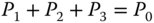
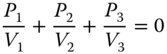
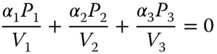
Thus, in the case of the achromatic doublet, judicious choice of glass pairs can minimise secondary colour, but without eliminating it. In principle, secondary colour can be entirely corrected in a triplet system employing lenses of different materials. More formally, if we describe the three lenses as having focal powers of P1, P2, and P3, with the Abbe numbers represented as V1, V2, and V3 and the partial dispersions as, α1, α2, α3, then the lens powers may be uniquely determined from the following set of equations:
As indicated previously, Figure 4.27 exemplifies the close link between primary and secondary dispersion, with a linear trend observed linking the partial dispersion and the Abbe number for most glasses. It is easy to demonstrate by presenting Eqs. (4.59a)–(4.59c) in matrix form that, if a wholly linear relationship exists between partial dispersion and Abbe number, then the matrix determinant will be zero. In this instance, a triplet solution is therefore impossible. Furthermore, the same analysis suggests that for a set of glasses lying close to a straight line on the partial dispersion plot will necessitate the deployment of lenses with very high countervailing powers. It is clear, therefore, that an optimum triplet design is afforded by selection of glasses that depart as far as possible from a straight-line plot on the partial dispersion diagram. In this context, the isolated group of glasses that appear in Figure 4.27, the fluorite glasses, are especially useful in correcting for secondary colour. These glasses lie particularly far from the general trend line for the ‘main series’ of glasses. Lenses which are corrected for both primary and secondary colour are referred to as apochromatic lenses. These lenses invariably incorporate fluorite glasses.
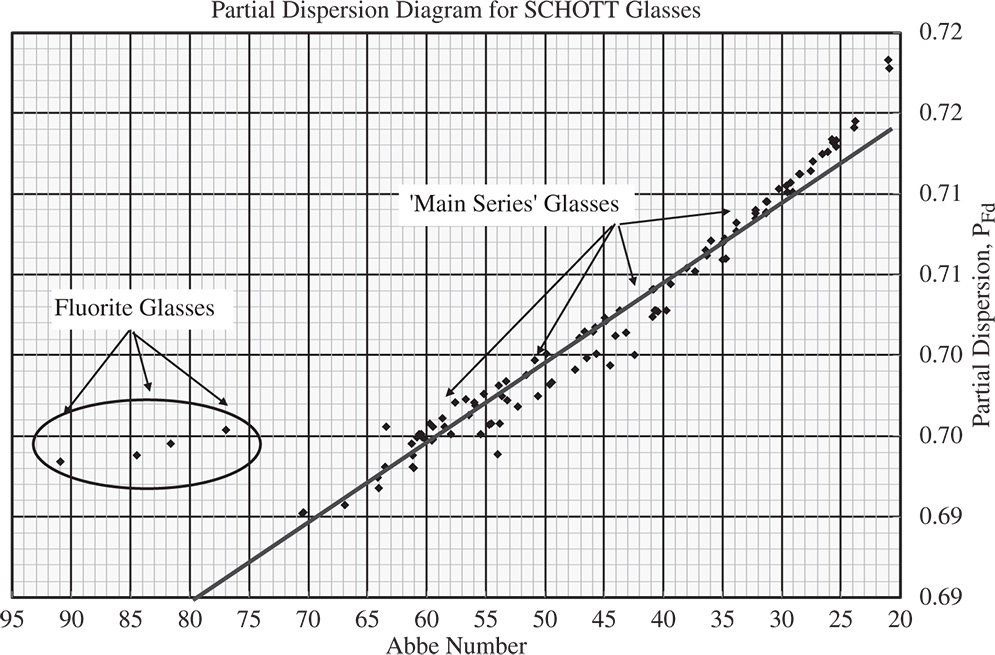
Figure 4.27 Plot of partial dispersion against Abbe number.
4.7.7 Spherochromatism
In the previous analysis we learned that the basic design of simple doublet lenses allowed for the correction of both chromatic aberration and spherical aberration. Furthermore, this flexibility for correction could be extended to coma for an air spaced lens. However, since the refractive index of the two glasses in a doublet lens varies with wavelength, then inevitably, so does the spherical aberration. As such, spherical aberration can only be corrected at one wavelength, e.g. at the ‘D’ wavelength. This means that there will be some uncorrected spherical aberration at the extremes of the spectrum. This effect is known as spherochromatism. It is generally less significant in magnitude when compared with secondary colour.
4.8 Hierarchy of Aberrations
For some specific applications, such as telescope and microscope objective lenses, the field angles tend to be very much smaller than the angles associated with the system numerical aperture. In these instances, the off-axis aberrations, such as coma, are much less significant than the on-axis aberrations. Therefore, as far as the Gauss-Seidel aberrations are concerned, there exists a hierarchy of aberrations that can be placed in order of their significance or importance:
i. Spherical Aberration
ii. Coma
iii. Astigmatism and Field Curvature
iv. Distortion
That is to say, it is of the greatest importance to correct spherical aberration and then coma, followed by astigmatism, field curvature, and distortion. This emphasises the significance and use of aplanatic elements in optical design.
Of course, for certain optical systems, this logic is not applicable. For instance, in both camera lenses and in eyepieces, the field angles are very substantial and comparable to the angles associated with the numerical aperture. Indeed, in systems of this type, greater emphasis is placed upon the correction of astigmatism, field curvature, and distortion than in other systems.
With these comments in mind, it would be useful to summarise all the aberrations covered in this chapter and to classify them by virtue of their pupil and field angle dependence. Table 4.1 sets out the wavefront error dependence upon pupil and field angle for each of the aberrations.
It would be instructive, at this point, to take the example of the 200 mm doublet and to plot the wavefront aberrations attributable to some of the aberrations listed in Table 4.1 against numerical aperture. Spherochromatism is expressed as the difference in spherical aberration wavefront error between the nF and nC wavelengths (486.1 and 656.3 nm). Secondary colour is expressed as the wavefront error attributable to the difference in defocus between the nF and nD wavelengths (486.1 and 589.3 nm). A plot is shown in Figure 4.28.
It is clear that for the simple achromat under consideration, at least for modest lens apertures, the impact of secondary colour predominates. If a wavefront error of about 50 nm is consistent with ‘high quality’ imaging, then secondary colour has a significant impact for numerical apertures in excess of 0.05 or f#10. With numerical apertures in excess of 0.2 (f#2.5), higher order spherical aberration starts to make a significant contribution. On the other hand the effect of spherochromatism is more modest throughout. In this context, the impact of spherochromatism would only be a significant issue if secondary colour were first corrected.
Table 4.1 Pupil and field dependence of principal aberrations.
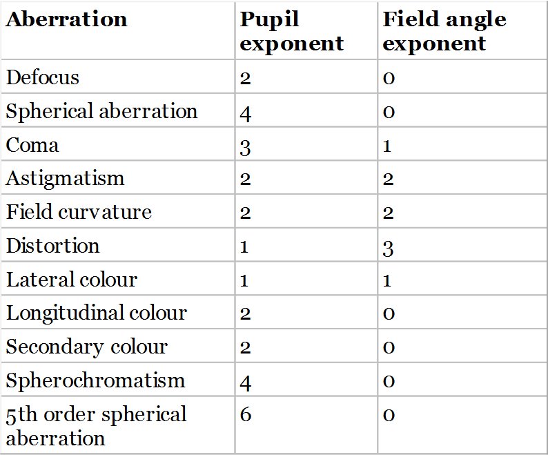
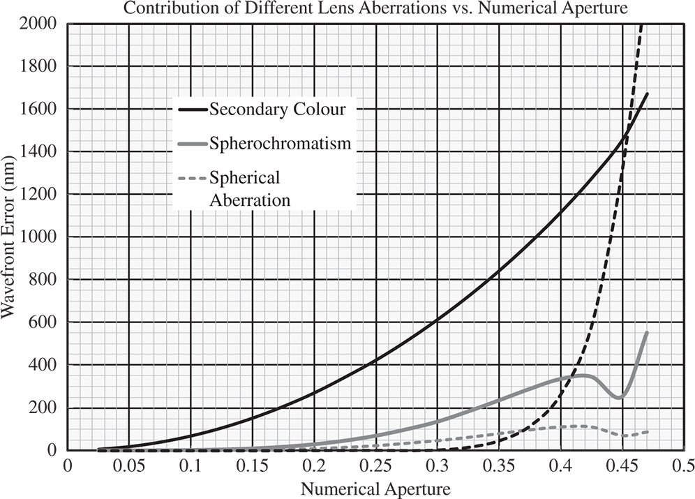
Figure 4.28 Contribution of different aberrations vs. numerical aperture for 200 mm achromat.
Of course, in practice, the design of such lens systems will be accomplished by means of ray tracing software or similar. Nonetheless, an understanding of the basic underlying principles involved in such a design would be useful in the initiation of any design process.
Further Reading
Born, M. and Wolf, E. (1999). Principles of Optics, 7e. Cambridge: Cambridge University Press. ISBN: 0-521-642221.
Hecht, E. (2017). Optics, 5e. Harlow: Pearson Education. ISBN: 978-0-1339-7722-6.
Kidger, M.J. (2001). Fundamental Optical Design. Bellingham: SPIE. ISBN: 0-81943915-0.
Kidger, M.J. (2004). Intermediate Optical Design. Bellingham: SPIE. ISBN: 978-0-8194-5217-7.
Longhurst, R.S. (1973). Geometrical and Physical Optics, 3e. London: Longmans. ISBN: 0-582-44099-8.
Mahajan, V.N. (1991). Aberration Theory Made Simple. Bellingham: SPIE. ISBN: 0-819-40536-1.
Mahajan, V.N. (1998). Optical Imaging and Aberrations: Part I. Ray Geometrical Optics. Bellingham: SPIE. ISBN: 0-8194-2515-X.
Mahajan, V.N. (2001). Optical Imaging and Aberrations: Part II. Wave Diffraction Optics. Bellingham: SPIE. ISBN: 0-8194-4135-X.
Slyusarev, G.G. (1984). Aberration and Optical Design Theory. Boca Raton: CRC Press. ISBN: 978-0852743577.
Smith, F.G. and Thompson, J.H. (1989). Optics, 2e. New York: Wiley. ISBN: 0-471-91538-1.
Welford, W.T. (1986). Aberrations of Optical Systems. Bristol: Adam Hilger. ISBN: 0-85274-564-8.
5
Aspheric Surfaces and Zernike Polynomials
5.1 Introduction
The previous chapters have provided a substantial grounding in geometrical optics and aberration theory that will provide the understanding required to tackle many design problems. However, there are two significant omissions.
Firstly all previous analysis, particularly with regard to aberration theory, has assumed the use of spherical surfaces. This, in part, forms part of a historical perspective, in that spherical surfaces are exceptionally easy to manufacture when compared to other forms and enjoy the most widespread use in practical applications. Modern design and manufacturing techniques have permitted the use of more exotic shapes. In particular, conic surfaces are used in a wide variety of modern designs.
The second significant omission is the use of Zernike circle polynomials in describing the mathematical form of wavefront error across a pupil. Zernike polynomials are an orthonormal set of polynomials that are bounded by a circular aperture and, as such, are closely matched to the geometry of a circular pupil. There are, of course, many different sets of orthonormal functions, the most well known being the Fourier series, which, in two dimensions, might be applied to a rectangular aperture. As the wavefront pattern associated with defocus forms one specific Zernike polynomial, the orthonormal property of the series means that all other terms are effectively optimised with respect to defocus. This topic was touched on in Chapter 3 when seeking to minimise the wavefront error associated with spherical aberration by providing balancing defocus. The optimised form that was derived effectively represents a Zernike polynomial.
5.2 Aspheric Surfaces
5.2.1 General Form of Aspheric Surfaces
In this discussion, we will restrict ourselves to surfaces that are symmetric about a central axis. Although more exotic surfaces are used, such symmetric surfaces predominate in practical applications. The most general embodiment of this type of surface is the so-called even asphere. Its general form is specified by its surface sag, z, which represents the axial displacement of the surface with respect to the axial position of the vertex, located at the axis of symmetry. The surface sag of an even asphere is given by the following formula:

c = 1/R is the surface curvature (R is the radius); k is the conic constant; αn is the even polynomial coefficient.
The curvature parameter, c, essentially describes the spherical radius of the surface. The conic constant, k, is a parameter that describes the shape of a conic surface. For k = 0, the surface is a sphere. More generally, the conic shapes are as set out in Table 5.1.
Table 5.1 Form of conic surfaces.