

Полная версия
Optical Engineering Science
In concentrating on third order aberrations, we shall, in the remainder of this chapter, seek to determine the impact of refractive surfaces, mirrors, and lenses on all the Gauss-Seidel aberrations. This analysis will proceed, initially, on the assumption that the surface in question lies at the pupil position. Subsequently, the impact of changing the position of the stop will be analysed. Manipulation of the stop position is an important variable in the optimisation of an optical design. The concept of the aplanatic geometry will be introduced where specific, simple optical geometries may be devised that are wholly free from either spherical aberration (SA) or coma (CO). These aplanatic building blocks feature in many practical designs and are significant because, in many instruments, such as telescopes and microscopes, there is a tendency for spherical aberration and coma to dominate the other aberrations. The elimination of spherical aberration and coma is thus a priority. Furthermore, by the same token, astigmatism (AS) and field curvature (FC) are more difficult to control. In particular, the control of field curvature is fundamentally limited by Petzval curvature, as alluded to in the previous chapter.
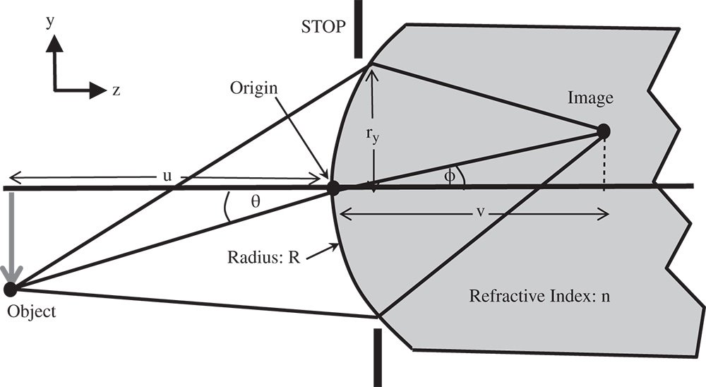
Figure 4.1 Calculation of OPD for refractive surface.
4.2 Aberration Due to a Single Refractive Surface
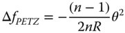
The analysis of the aberrations of a single refractive surface is based on the computation of the OPD of a generalised field point to the appropriate order (4th) in terms of field angle, θ and ray height, r, at the pupil. For this analysis, we will assume that the pupil is located at the lens surface. In calculating the OPD, we force all rays to go to the paraxial focus and compute the OPD with respect to the chief. Figure 4.1 shows an object with a field angle, θ, located at a distance, u from a spherical refractive surface of radius R. It must be emphasised, in this instance, that this analysis applies specifically to a spherical surface. In this geometry, it is assumed that the object is displaced from the optical axis in the y direction. The paraxial image is itself located at a distance v from the surface and the position of a ray at the surface (and stop) is described by its components in x and y – hx and hy.
The image in this case is the paraxial image and from the paraxial theory, the angle φ may be expressed in terms of θ as θ/n. To compute the optical path of a general ray as it passes from object to paraxial image, we need to define the ray co-ordinates at three points:


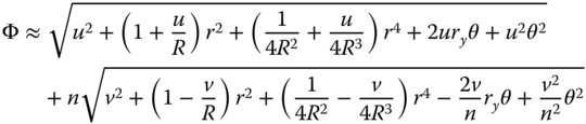
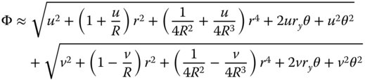
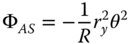
The z co-ordinate of the stop position is derived from the binomial expansion for the axial sag of a sphere including terms up to the fourth power. In making this approximation, it is assumed that h is significantly less than R. If we were to adopt the paraxial approximation we would only consider the first r2 term in the expansion. In the case of third order aberration, we need to consider the next term. It is then very straightforward to calculate the total optical path, Φ, for a general ray in passing from object to paraxial image:

The two square root terms represent the optical path of two ‘legs’ of the journey, with the path through the glass adding a multiplicative factor of n. The next stage of the process is an extension of the paraxial theory. It is assumed that rx, ry, and uθ are all significantly less than u. We can now approximate Φ from Eq. (4.2) using the binomial theorem. In the meantime collecting terms we get:
Before deriving the third order aberration terms, we examine the paraxial contribution which contain terms in h up to order r2.

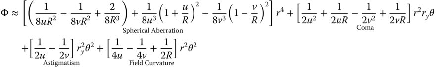
As one would expect, in the paraxial approximation, the optical path length is identical for all rays. However, for third order aberration, terms of up to order h4 must be considered. Expanding Eq. (4.2) to consider all relevant terms, we get:
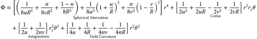
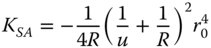
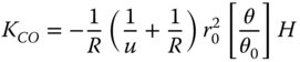
Four of the five Gauss-Seidel terms are present – spherical aberration, coma, astigmatism, and field curvature. However, clearly there is no distortion. In fact, as will be seen later, distortion can only occur where the stop is not at the surface as it is here. Of course, Eq. (4.4) can be simplified if one considers that u, v, and R are dependent variables, as related in Eq. (4.3). Substituting v for u, and R, we can express the OPD in terms of u and R alone. Furthermore, it is useful, at this stage to split the OPD contributions in Eq. (4.4) into Spherical Aberration (SA), Coma (CO), Astigmatism (AS), and Field Curvature (FC). With a little algebraic manipulation this gives:

4.2.1 Aplanatic Points
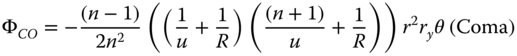
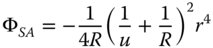
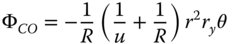
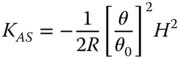
It is worthwhile, at this juncture, to examine the four expressions in Eqs. (4.5a)–(4.5d) in some detail and, in particular, those for spherical aberration and coma. Before examining these expressions further, it is worthwhile to cast them in the form outlined in Chapter 3:
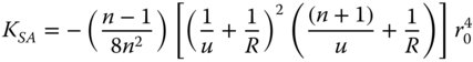
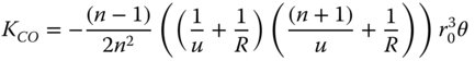
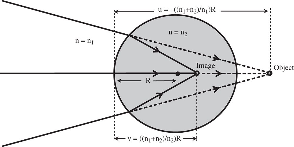
Figure 4.2 Aplanatic points for refraction at single spherical surface.
There is a clear pattern in these expressions in that both spherical aberration and coma can be reduced to zero for specific values of the object distance, u. Examining Eqs. (4.6a) and (4.6b), it is evident that this condition is met where u = −R. That is to say, where the object is located at the centre of the spherical surface. However, this is a somewhat trivial condition where rays are undeviated by the surface and where the surface would not provide any useful additional refractive power to the system. Most significantly, another condition does exist for u = −(n + 1)R. Here, for this non-trivial case, both third order spherical aberration and coma are absent. This is the so-called aplanatic condition and the corresponding conjugate points are referred to as aplanatic points (Figure 4.2). From Eq. (4.3) we can derive the image distance, v, as (n + 1)R/n. That is to say, the object is virtual and the image is real if R is positive and vice-versa if R is negative.
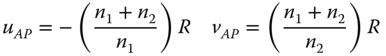
To be a little more rigorous, we might suppose that refractive index in object space is n1 and that in image space is n2. The location of the aplanatic points is then given by:
Fulfilment of the aplanatic condition is an important building block in the design of many optical systems and so is of great practical significance. As pointed out in the introduction, for those systems where the field angles are substantially less than the marginal ray angles, such as microscopes and telescopes, the elimination of spherical aberration and coma is of primary importance. Most significantly, not only does the aplanatic condition eliminate third order spherical aberration, but it also provides theoretically perfect imaging for on axis rays.
Worked Example 4.1 Microscope Objective
The ‘front end’ of many high power microscope objectives exploits the principle of single surface aplanatic points through the use of a hyperhemisphere co-located with the object. The hyperhemisphere consists of a sphere that has been truncated at one of the aplanatic points which also coincides with the object location, as illustrated in Figure 4.3.
Using the hyperhemisphere, we wish to create a ×20 microscope objective for a standard optical tube length of 200 mm. In this example, it is assumed that two thirds of the optical power resides in the hyperhemisphere itself; other components collimate the beam. In other words:
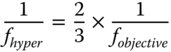
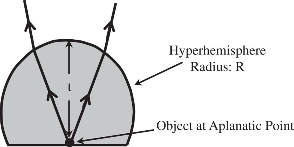
Figure 4.3 Hyperhemisphere objective.
The refractive index of the hyperhemisphere is 1.6. What is the radius, R, of the hyperhemisphere and what is its thickness?
For a tube length of 200 mm, a ×20 magnification corresponds to an objective focal length of 10 mm. As two thirds of the power resides in the hyperhemisphere, then the focal length of the hyperhemisphere must be 15 mm. Inspecting Figure 4.2, it is clear that the thickness of the hyperhemisphere is −R × (n + 1)/n, or −1.625 × R. To calculate the value of R, we set up a matrix for the system. The first matrix corresponds to refraction at the planar air/glass boundary, the second to translation to the spherical surface and the final matrix to the refraction at that surface. On this occasion, translation to the original reference is not included.
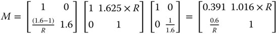
From the above matrix, the focal length is −R/0.6 and hence R = −9.0 mm. The thickness, t, we know is −1.625 × R and is 14.625. In this sign convention, R is negative, as the sense of its sag is opposite to the direction of travel from object to image space.
The (virtual) image is at (n + 1) × R from the sphere vertex or 2.6 × 9 = 23.4 mm.
In summary:

4.2.2 Astigmatism and Field Curvature
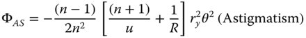
Unlike spherical aberration and coma, there is less scope for correction of astigmatism and field curvature. In Eqs. (4.5c) and (4.5d), astigmatism is corrected at the aplanatic point and field curvature at the radial points. However, the convention used in Eq. (4.5c) to describe astigmatic correction corresponds to zero sagittal ray defocus. On the other hand, using the alternative convention set out in Chapter 3 we have:
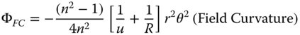
From Eq. (4.8a), it is evident that at the aplanatic condition where u = −(n + 1)R, the astigmatism vanishes, as does the spherical aberration and coma. It is interesting to see what might happen to the field curvature where this condition is fulfilled:
This is related to the Petzval field curvature, which, by definition, is the field curvature that arises when the astigmatism in the system is zero. Relating this to Eq. 4.8b, then the field curvature may be expressed as:
Figure 4.4 Field curvature for single refraction.
It is clear that Eq. (4.9) represents, with its quadratic dependence upon the pupil location, r, a degree of defocus, Δf, or longitudinal aberration, that is quadratic in the field angle. This defocus is given by:
The systematic field dependent defocus can be represented as a spherical surface where the each field point is in focus. The curvature of this surface, CPETZ and equivalent to 1/RPETZ where RPETZ is the Petzval Radius, is given by:
The sign is important, in that the Petzval curvature is in the opposite sense to that of the surface itself. This point is illustrated in Figure 4.4.
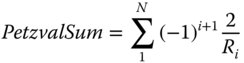
The most significant point about Petzval curvature is, in common with the underlying wavefront error, that it is additive through a system. To illustrate this, we might consider a system with N surfaces with radius of curvature Ri. The material that follows each surface has a refractive index of ni. The Petzval curvature associated with the system is simply the sum of the individual curvatures and is referred to as the Petzval sum. This is given by:
The practical implication of Eq. (4.13) is that if a system consists of elements with entirely positive or entirely negative focal power, then that system will always exhibit field curvature. To achieve a flat field, or a zero Petzval sum, then any positive optical elements must be balanced by negative elements elsewhere in the system.
It must be emphasised that the condition for perfect image formation on the Petzval surface applies specifically to the scenario where astigmatism has been removed.
4.3 Reflection from a Spherical Mirror
The third order analysis for a spherical mirror proceeds in very much the same way as the single refractive surface. That is to say, a ray is traced from the object location to the mirror and thence to the paraxial focus regardless as to whether the real ray actually terminates there. The general layout is shown in Figure 4.5. The sign convention used here is the same as applied to all previous analyses. That is to say, positive image distance is with the image to the right, and the image distance, as shown in Figure 4.5, is actually negative. However, it must be accepted that, as rays physically converge on this image point, then this image is actually real, despite v being negative. In addition, the same convention is applied to mirror curvature; the mirror depicted in Figure 4.5 has negative curvature.
Figure 4.5 Reflection at spherical mirror.
The analysis proceeds as previously. Firstly, we set out the object and image positions and the ray intercept at the stop.


The optical path is given by:

Rearranging:
In applying the binomial approximation, one needs to be careful with regard to the sign convention. It should be accepted that each of the square root terms in Eq. (4.14) is positive for a real object and real image. That is to say, all rays are physically traced to the appropriate location. In the case of a mirror surface, the definition of a real image corresponds to a negative image distance, u. Once again, we examine the paraxial terms

As for the refractive surface we expand Eq. (4.14) using the binomial theorem to give terms of the fourth order in OPD.
As with the refractive case, four of the five Gauss-Seidel terms are present – spherical aberration, coma, astigmatism, and field curvature. There is also no distortion. As previously, Eq. (4.16) can be simplified considering u, v, and R as dependent variables, as related in Eq. (4.15). We can, once more, express the OPD in terms of u and R alone. Splitting the OPD contributions in Eq. (4.16) into Spherical Aberration (SA), Coma (CO), Astigmatism (AS), and Field Curvature (FC) and with a little algebraic manipulation we have:

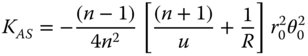
Equations (4.17a)–(4.17c) bear some striking similarities with respect to those for the refractive surface. In fact, if one substitutes n = −1 in the corresponding refractive formulae, one obtains expressions similar to those listed above. Thus, in some ways, a mirror behaves as a refractive surface with a refractive index of minus one. Once again, there are aplanatic points where both spherical aberration and coma are zero. This occurs only where both object and image are co-located at the centre of the spherical surface. The apparent absence of field curvature may appear somewhat surprising. However, the Petzval curvature is non-zero, as will be revealed. We can now cast all terms in the form set out in Chapter 3 and introduce the Lagrange invariant, which is equal to the product of r0 and θ0 (the maximum field angle):
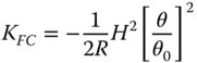
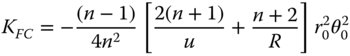
The Petzval curvature is simply given by subtracting twice the KAS term in Eq. (4.18c) from the field curvature term in Eq. (4.18d). This gives:
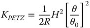
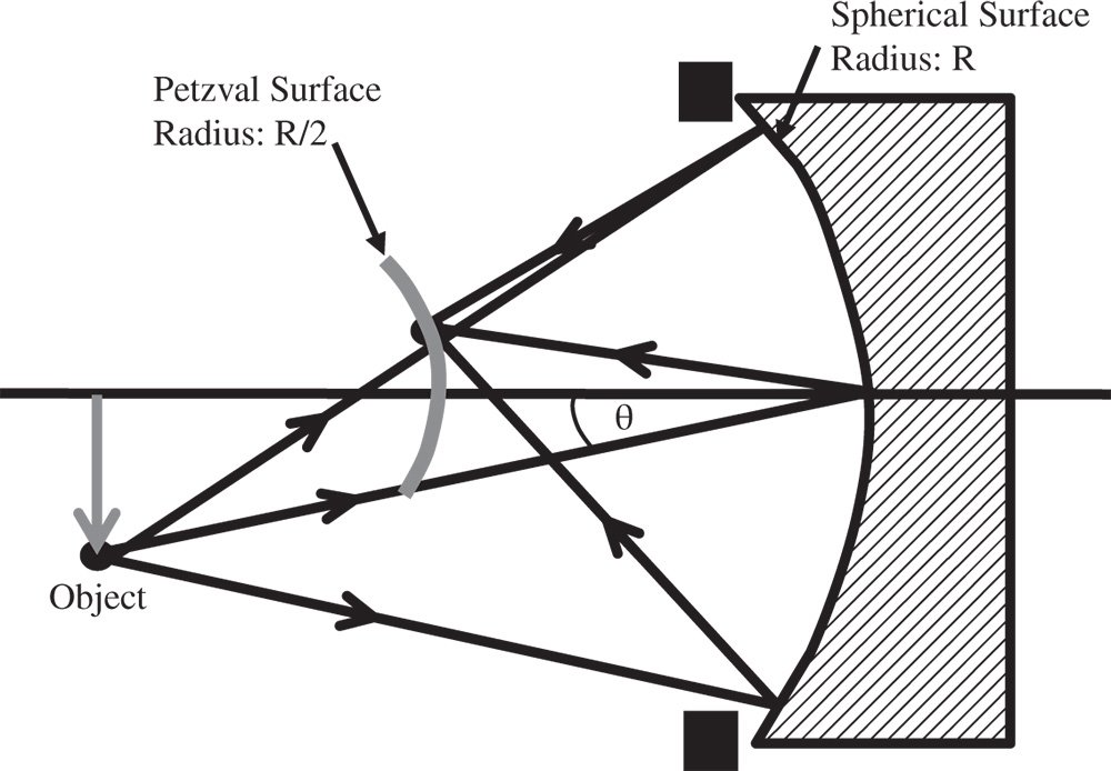
Figure 4.6 Petzval curvature for mirror.
In this instance, the Petzval surface has the same sense as that of the mirror itself. However, the radius of the Petzval surface is actually half that of the original surface. This is illustrated in Figure 4.6.
Calculation of the Petzval sum proceeds more or less as the refractive case. However, there is one important distinction in the case of a mirror system. For a system comprising N mirrors, each successive mirror surface inverts the sense of the wavefront error imparted by the previous mirrors.
4.4 Refraction Due to Optical Components
4.4.1 Flat Plate
Equations (4.5a)–(4.5d) give the Gauss-Seidel aberration terms for a spherical reflector. However, for a flat surface, where 1/R = 0, the aberration is non zero.

If we now make the approximation that r0/u∼NA0 and express all wavefront errors in terms of the normalised pupil function, we obtain the following expressions.
In all expressions, the wavefront error is proportional to the object distance. Equation 4.22 only considers refraction at a single surface. For a flat plate whose thickness is vanishingly small, it is clear that refraction at the second (glass-air) boundary will produce a wavefront error that is equal and opposite to that induced at the first surface. Furthermore, it is also clear that the form of wavefront error contribution will be identical to Eq. (4.22), but reversed in sign. For a glass plate of finite thickness, t, the effective object distance, expressed as the object distance in air, will be given by u + t/n. Therefore, the relevant wavefront error contributions at the second surface are given by:


The total wavefront error is then simply given by the sum of the two contributions. This is expressed in standard format, as below:

The important conclusion here is that a flat plate will add to system aberration, unless the optical beam is collimated (object at infinite conjugate). This is of great practical significance in microscopy, as a thin flat plate, or ‘cover slip’ is often used to contain a specimen. A standard cover slip has a thickness, typically, of 0.17 mm. Examination of Eq. (4.24) suggests that this cover slip will add significantly to system aberration. In practice, it is the spherical aberration that is of the greatest concern, as θ0 is generally much smaller than NA0 in most practical applications. As a consequence, some microscope objectives are specifically designed for use with cover slips and have built in aberration that compensates for that of the cover slip. Naturally, a microscope objective designed for use with a cover slip will not produce satisfactory imaging when used without a cover slip.
Worked Example 4.2 Microscope Cover Slip
A microscope cover slip 0.17 mm thick is to be used with a microscope objective with a numerical aperture of 0.8. The refractive index of the cover slip is 1.5. What is the root mean square (rms) spherical aberration produced by the cover slip? The aberration is illustrated in Figure 4.7.
From Eq. (4.24):

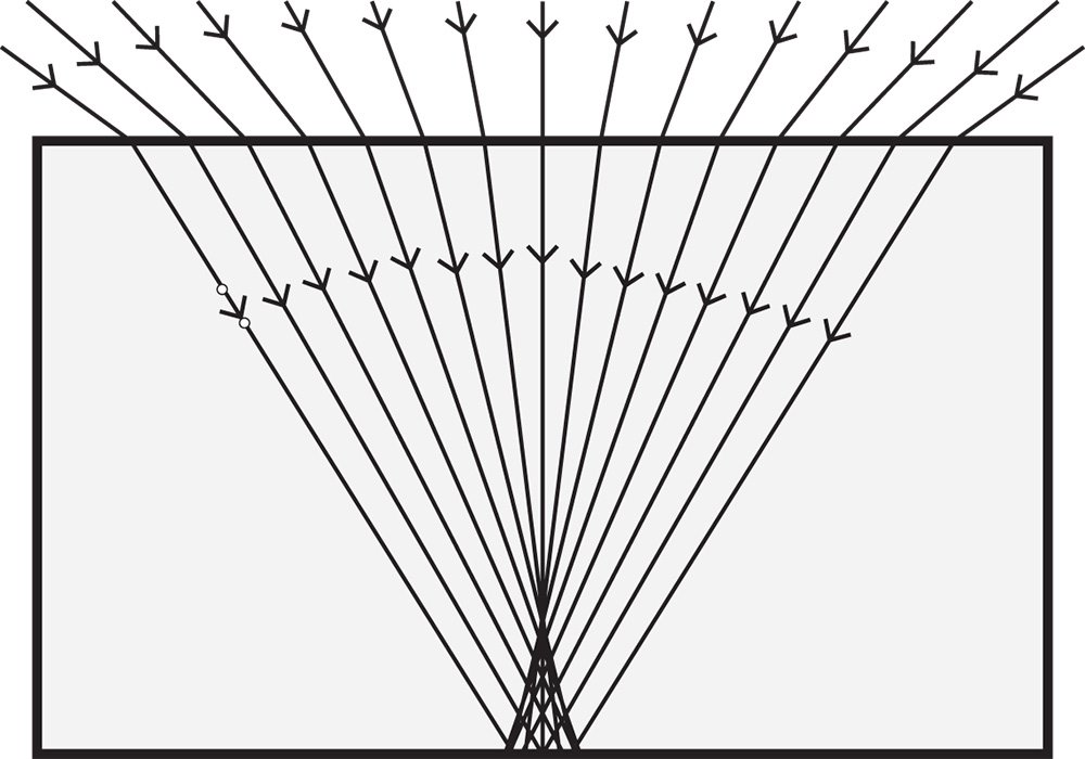
Figure 4.7 Spherical aberration in cover slip.
Substituting the above values we get: Ksa = 0.003 22 mm or 3.2 μm.
The wavefront error (in microns) is thus given by:

where p is the normalised pupil function.
For reasons that will become apparent later, in practice, wavefront errors are usually expressed as a fraction of some standard wavelength, for example 589 nm. The above wavefront error represents about 0.4 × λ when expressed in this way. An rms wavefront error of about λ/14 is considered consistent with good image quality. This level of aberration is, therefore, significant and measures must be taken (within the objective) to correct for it.