


Полная версия
Optical Engineering Science
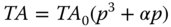
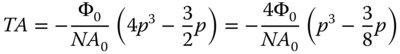
TA0 is the nominal third order aberration and α represents the defocus
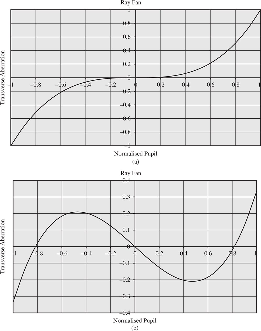
Figure 3.3 (a) Ray fan for pure third order aberration. (b) Ray fan with third order aberration and defocus.
Since the geometry is assumed to be circular, to calculate the rms (root mean square) aberration, one must introduce a weighting factor that is proportional to the pupil function, p. The mean squared transverse aberration is thus:
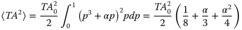
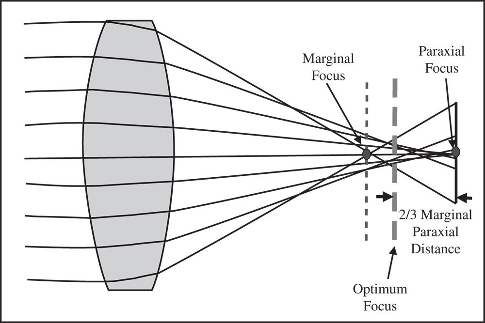
Figure 3.4 Balancing defocus against aberration – optimal focal position.
The expression is minimised where α = −2/3. To understand the significance of this, examination of Eq. (3.6) suggests that, without defocus, the marginal ray (p = 1) has a longitudinal aberration of TA0/NA. The defocus term itself produces a constant longitudinal aberration or defocus of αTA0/NA. Therefore, the optimum defocus is equivalent to placing the adjusted focus at 2/3 of the distance between the paraxial and marginal focus, as shown in Figure 3.4. Without this focus adjustment, with the third order aberration viewed at the paraxial focus, the rms aberration is TA0/4. However, adding the optimum defocus reduces the rms aberration to TA0/12, a reduction by a factor of 3.
This analysis provides a very simple introduction to the concept of third order aberrations. In the basic illustration so far considered, we have looked at the example of a simple lens focussing an on axis object located at infinity. In the more general description of monochromatic aberrations that we will come to, this simple, on-axis aberration is referred to as spherical aberration. In developing a more general treatment of aberration in the next sections we will introduce the concept of optical path difference (OPD).
3.3 Aberration and Optical Path Difference
In the preceding section, we considered the impact of optical imperfections on the transverse aberration and the construction of ray fans. Unfortunately, this treatment, whilst providing a simple introduction, does not lead to a coherent, generalised description of aberration. At this point, we introduce the concept of optical path difference (OPD). For a perfect imaging system, with no aberration, if all rays converge onto the paraxial focus, then all ray paths must have the same optical path length from object to image. This is simply a statement of Fermat's principle. We now consider an aberrated system where we accurately (not relying on the paraxial approximation) trace all rays through the system from object to image. However, at the last surface, we (hypothetically) force all rays to converge onto the paraxial focus. For all rays, we compute the optical path from object to image. The OPD is the difference between the integrated optical path of a specified ray with respect to the optical path of the chief ray. Of course, if there were no aberration present, the OPD would be zero. Thus, the OPD represents a quantitative description of the violation of Fermat's principle.
The general concept is shown in Figure 3.5. Rays are accurately traced from the object through the system, emerging into image space. That is to say, ray tracing proceeds until the last optical surface, mirror or lens etc. Following the preceding discussion, at some point, we force all rays to converge upon the paraxial focus. However, the convention for computing OPD is that all rays are traced back to a spherical surface centred on the paraxial focus and which lies at the exit pupil of the system. Of course, it must be emphasised that the real rays do not actually follow this path. In the generic system illustrated, the real ray is traced to point P located in object space and the optical path length computed. Thereafter, instead of tracing the real ray into the object space, a dummy ray is traced, as shown by the dotted line. This dummy ray is traced from point P to point Q that lies on the reference surface – a sphere located at the exit pupil and centred on the paraxial focus. The optical path length of this segment is then added to the total.
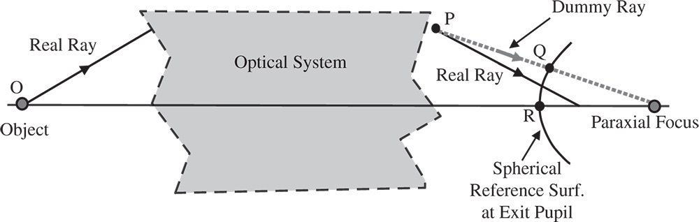
Figure 3.5 Illustration of optical path difference.
After calculating the optical path length for the dummy ray OPQ, we need to calculate the OPD with respect to the chief ray. The chief ray path is calculated from the object to its intersection with the reference sphere at the pupil, represented, in this instance, by the path OR. In calculating the OPD, the convention is that the OPD is the chief ray optical path (OR) minus the dummy ray optical path (OPQ). Note the sign convention.

Having established an additional way of describing aberrations in terms of the violation of Fermat's principle, the question is what is the particular significance and utility of this approach? The answer is that, when expressed in terms of the OPD, aberrations are additive through a system. As a consequence of this, this treatment provides an extremely powerful general description of aberrations and, in particular, third order aberrations. Broadly, aberrations can be computed for individual system elements, such as surfaces, mirrors, or lenses and applied additively to the system as a whole. This generality and flexibility is not provided by a consideration of transverse aberrations.
There is a correspondence between transverse aberration and OPD. This is illustrated in Figure 3.6. At this point, we introduce a concept that is related to that of OPD, namely wavefront error(WFE). We must remember that, according to the wave description, the rays we trace through the system represent normals to the relevant wavefront. The wavefront itself originates from a single object point and represents a surface of equal phase. As such, the wavefront represents a surface of equal optical path length. For an aberrated optical system, the surface normals (rays) do not converge on a single point. In Figure 3.6, this surface is shown as a solid line. A hypothetical spherical surface, shown as a dashed line, is now added to represent rays converging on the paraxial focus. This surface intersects the real surface at the chief ray position. The distance between these two surfaces is the WFE.
In terms of the sign convention, the wavefront error, WFE, is given by:

The sign convention is important, as it now concurs with the definition of OPD. As the wavefronts form surfaces of constant optical path length, there is a direct correspondence between OPD and WFE. A positive OPD indicates the optical path of the ray at the reference sphere is less than that of the chief ray. Therefore, this ray has to travel a small positive distance to ‘catch up’ with the chief ray to maintain phase equality. Hence, the WFE is also positive.
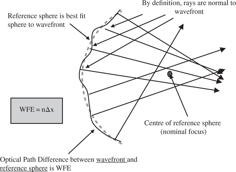
Figure 3.6 Wavefront representation of aberration.
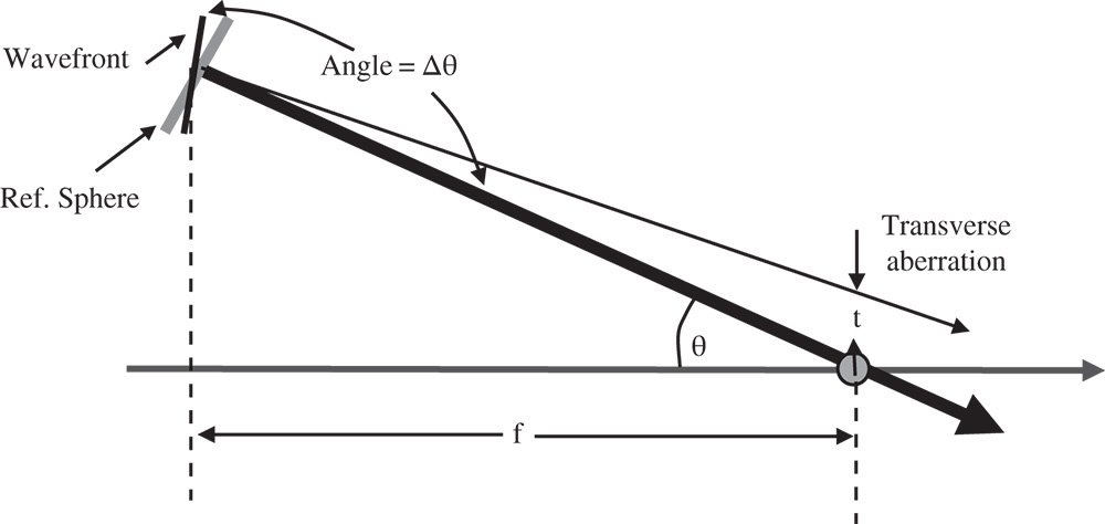
Figure 3.7 Simplified wavefront and ray geometry.
Both OPD and WFE quantify the violation of Fermat's principle in the same way. OPD is generally used to describe the path length difference of a specific ray. WFE tends to be used when describing OPD variation across an assembly of rays, specifically across a pupil. The concept of WFE enables us to establish the relationship between OPD and transverse aberration in that it helps define the link between wave (phase and path length) geometry and ray geometry. This is shown in Figure 3.7. It is clear that the transverse aberration is related to the angular difference between the wavefront and reference sphere surfaces.
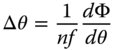
We now describe the WFE, Φ, as a function of the reference sphere (paraxial ray) angle, θ. The radius of the reference sphere (distance to the paraxial focus) is denoted by f. This allows us to calculate the difference in angle, Δθ, between the real and paraxial rays. This is simply equal to the difference in local slope between the two surfaces.
n is the medium refractive index.
In this analysis, the WFE represents the difference between the real and reference surfaces with the positive axial direction represented by the propagation direction (from object to image). In this convention, the WFE has the opposite sign to the OPD. The transverse aberration, t, can be derived from simple trigonometry.
If θ describes the angle the ray makes to the chief ray, then Eq. (3.10) may be reformed in terms of the numerical aperture, NA. The numerical aperture is equal to nsinθ, and Eq. (3.11) may be recast as:
So, the transverse aberration may be represented by the first differential of the WFE with respect to the numerical aperture. In terms of third order aberration theory, the numerical aperture of an individual ray is directly proportional to the normalised pupil function, p. If the overall system, or marginal ray, numerical aperture is NA0, then the individual ray numerical aperture is simply NA0p. The transverse aberration is then given by:
Equation (3.12) provides a simple direct relationship between OPD and transverse aberration. Of course, we know that, for third order aberration, the transverse aberration is proportional to the third power of the pupil function, p. If this is the case, then it is apparent, from Eq. (3.12), that the OPD is proportional to the fourth power of the pupil function. So, for third order aberration, the transverse aberration shows a third power dependence upon the pupil function whereas the OPD shows a fourth power dependence.
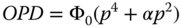
Applying these arguments to the analysis of the simple on-axis example illustrated earlier, with the object placed at the infinite conjugate, then the WFE can be represented by the following equation:
p is the normalised pupil function.
Figure 3.8 shows a plot of the OPD against the normalised pupil function; such a plot is referred to as an OPD fan.
Despite the fact that this simple aberration has a quartic dependence on the pupil function, it is still referred to as third order aberration after the transverse aberration dependence. As with the optimisation of transverse aberration, the OPD can be balanced by applying defocus to offset the aberration. We saw earlier that a simple defocus produces a linear term in the transverse aberration. Referring to Eq. (3.12), it is clear that defocus may be represented by a quadratic term. Equation (3.14) describes the OPD when some defocus has been added to the initial aberration.
An OPD fan with aberration plus balancing defocus is shown in Figure 3.9.
In this instance, the plot has a characteristic ‘W’ shape, with the curve in the vicinity of the origin dominated by the quadratic defocus term. As with the case for transverse aberration, the defocus can be optimised to produce the minimum possible OPD value when taken as a root mean squared value over the circular pupil. Again, using a weighting factor that is proportional to the pupil function, p, (to take account of the circular geometry), the mean squared OPD is given by:
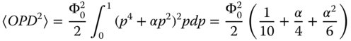
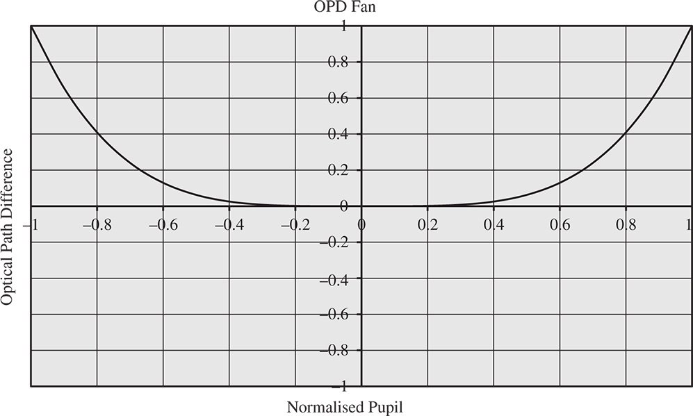
Figure 3.8 Quartic OPD fan.
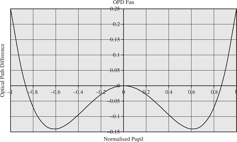
Figure 3.9 OPD fan with balancing defocus.
The above expression has a minimum where α = −¾. To understand the magnitude of this defocus, it is useful first to convert the new OPD expression into a transverse aberration using Eq. (3.12).
From Eq. (3.16), it can be seen that the optimum defocus is 3/8 of the distance between the paraxial and marginal ray foci. This value is different to that derived for the optimisation of the transverse aberration itself. It should be understood that the optimisation of the transverse aberration and the OPD, although having the same ultimate purpose in minimising the aberration, nonetheless produce different results. Indeed, in the optimisation of optical designs, one is faced with a choice of minimising either the geometrical spot size (transverse aberration) or OPD in the form of rms WFE. The rationale behind this selection will be considered in later chapters when we examine measures of image quality, as applied to optical design.
The balanced defocus, as illustrated in Eq. (3.15) does significantly reduce the rms OPD. In fact, it reduces the OPD by a factor of four. Resultant rms values are set out in Eq. (3.17).

3.4 General Third Order Aberration Theory
Armed with a simple understanding of the basic concepts that lie behind the description of third order aberration, we can proceed to a more general and more powerful analysis. This analysis relies on a theoretical treatment of OPD as a measure of aberration. As pointed out earlier, although the lowest order aberration (beyond the paraxial approximation) has a fourth order dependence upon pupil function, this theory is still referred to as third order aberration theory. In the example we have hitherto considered, we have analysed an on axis object located at the infinite conjugate. For the more general treatment, we must consider off-axis objects with the chief ray having some non-zero field angle with respect to the optical axis. In addition, the object may have an arbitrary axial location and we must also consider the axial position of the pupil.
This third order theory is referred to as Gauss-Seidel aberration theory and is of general applicability to optical systems of arbitrary complexity. There is, however, one important constraint. The theory assumes that the entire geometry, component surfaces and so on, is circularly symmetric about the optical axis. In formulating the theory, we assume that the object presents a non-zero field angle, θ, with respect to the optic axis which is assumed to be oriented along the z axis. The chief ray is tilted by rotation about the x axis, so the object is offset from the optical axis in the y direction. The third order aberrations are to be expressed in terms of the field angle, θ, and the normalised pupil function, p. However, in this instance, because of the non-zero field angle, the rotational symmetry of the pupil is removed, so that separate x and y components of the pupil function, px, py, must be introduced.
The assumption in the Gauss-Seidel theory is that the underlying third order aberrations in a symmetrical optical system are themselves symmetrical and proportional to the fourth power of the pupil function. However, the finite field angle will effectively introduce an offset in the effective y component of the pupil function, Δpy, at some arbitrary optical component. This is illustrated in Figure 3.10 which shows generically how such an offset may be visualised.
What is suggested by Figure 3.10 is that if a co-ordinate transformation is applied in y that is proportional to the field angle, θ, then the ray fan can be made symmetrical about this new optical axis. That is to say, in Figure 3.10b, any aberration generated would, in terms of OPD, simply be proportional to p4, with respect to the new axis. In arguing that the required offset is proportional to θ, rather than some other trigonometrical function, we are making an approximation based on linearization in θ. This is justified for third order analysis, since any error produced would only be visible in higher order aberration terms (than third order). In Figure (3.10), the pupil is shown at the optical surface under consideration. However, this is not a necessary condition; wherever the pupil is located a symmetrical ray fan may be produced by simple offset of the co-ordinate system in the Y axis.
Thus, by the argument presented here, any third order aberration may be represented by a pupil dependence of p4 augmented by a shift in the y component of the pupil function, Δpy that is proportional to the field angle, θ. This is set out in Eq. (3.18), which describes the WFE, Φ, in terms of θ, p, and py. From this point, we use WFE, rather than OPD as the key descriptor, as we are describing OPDs across the entire pupil. The offset pupil is now denoted by p′
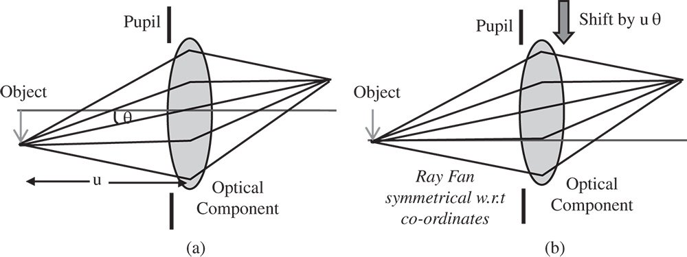
Figure 3.10 (a) Generic layout. (b) Layout with y co-ordinate transformation.
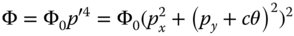
c is a constant of proportionality for the pupil offset.
Equation 3.18 may be expanded as follows:

Finally expanding Eq. (3.19) gives an expression for all third order aberrations:

Equation (3.20) contains six distinct terms describing the WFE across the pupil. However, the final term, c4θ4, for a given field position, simply describes a constant offset in the optical path or phase of the rays originating from a particular point. That is to say, for a specific ray bundle, no OPD or violation of Fermat's principle could be ascribed to this term, when the difference with respect to the chief ray is calculated. Therefore, the final term in Eq. (3.20) cannot describe an optical aberration. We are thus left with five distinct terms describing third order aberration, each with a different dependence with respect to pupil function and field angle. These are the so called five third order Gauss-Seidel aberrations. Of course, in terms of the WFE dependence, all terms show a fourth order dependence with respect to a combination of pupil function and field angle. That is to say, the sum of the exponents in p and in θ must always sum to 4.
3.5 Gauss-Seidel Aberrations
3.5.1 Introduction
In this section we will describe each of the fundamental third order aberrations in turn. Re-iterating Eq. (3.20) below, it is possible to highlight each of the aberration terms:

We will now describe each of these five terms in turn.
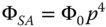
3.5.2 Spherical Aberration
The first term, spherical aberration, has a simple fourth order dependence upon pupil function and no dependence upon field. This is illustrated in Eq. (3.21):
This aberration shows no dependence upon field angle and no dependence upon the orientation of the ray fan. Since, in the current analysis and for a non-zero field angle, the object is offset along the y axis, then the pupil orientation corresponding to py defines the tangential ray fan and the pupil orientation corresponding to px defines the sagittal ray fan. This is according to the nomenclature set out in Chapter 2. So, the aberration is entirely symmetric and independent of field angle. In fact, the opening discussion in this chapter was based upon an illustration of spherical aberration.
Spherical aberration characteristically produces a circular blur spot. The transverse aberration may, of course, be derived from Eq. (3.21) using Eq. (3.12). For completeness, this is re-iterated below:
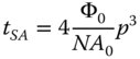
A 2D geometrical plot, of ray intersection at the paraxial focal plane, as produce by an evenly illuminated entrance pupil is referred to as a geometrical point spread function. Due to the symmetry of the aberration, this spot is circular. However, since the transformation in Eq. (3.22) is non-linear, the blur spot associated with spherical aberration is non uniform. For spherical aberration alone (no defocus or other aberrations), the density of the geometrical point spread function is inversely proportional to the pupil function, p. That is to say, spherical aberration manifests itself as a blur spot with a pronounced peak at the centre, with the density declining towards the periphery. This is illustrated in Figure 3.11. The spot, as shown in Figure 3.11, with a pronounced central maximum, is characteristic of spherical aberration and should be recognised as such by the optical designer.
As suggested earlier, the size of this spot can be minimised by moving away from the paraxial focus position. The ray fan and OPD fan for this aberration look like those illustrated in Figures 3.3 and 3.8. Overall, the characteristics of spherical aberration and the balancing of this aberration is very much as described in the treatment of generic third order aberration, as set out earlier.
Figure 3.11 Geometrical spot associated with spherical aberration.
3.5.3 Coma
The second term, coma, has an WFE that is proportional to the field angle. Its pupil dependence is third order, but it is not symmetrical with respect to the pupil function. The WFE associated with coma is as below:
In the preceding discussions, the transverse aberration has been presented as a scalar quantity. This is not strictly true, as the ray position at the paraxial focus is strictly a vector quantity that can only be described completely by an x component, tx and a y component ty. Equation (3.12) should strictly be rendered in the following vectorial form:
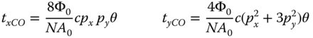
The transverse aberration relating to coma may thus be written out as:
From the perspective of both the OPD and ray fans the behaviour of the tangential (y) and sagittal ray fans are entirely different. As an optical designer, the reader should ultimately be familiar with the form of these fans and learn to recognise the characteristic third order aberrations. For a given field angle, the tangential OPD fan (px = 0) shows a cubic dependence upon pupil function, whereas, for the sagittal ray fan (py = 0), the OPD is zero. The OPD fan for coma is shown below in Figure 3.12.
The picture for the ray fans is a little more complicated. For both the tangential and sagittal ray fans, there is no component of transverse aberration in the x direction. On the other hand, for both ray fans, there is a quadratic dependence with respect to pupil function for the y component of the transverse aberration. The problem, in essence, it that transverse aberration is a vector quantity. However, when ray fans are computed for optical designs they are presented as scalar plots for each (tangential and sagittal) ray fan. The convention, therefore, is to plot only the y (tangential) component of the aberration in a tangential ray fan, and only the x (sagittal) component of the aberration in a sagittal ray fan. With this convention in mind, the tangential ray fan shows a quadratic variation with respect to pupil function, whereas there is no transverse aberration for the sagittal ray fan. Tangential and sagittal ray fan behaviour is shown in Figure 3.13 which shows relevant plots for coma.