

Полная версия
Optical Engineering Science
For the two cases illustrated in Figure 2.7, the eye's focussing power remains the same. Therefore, addition of a lens of focal length f will change the closest approach distance, d0, to:
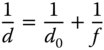
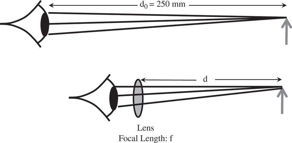
Figure 2.7 Simple magnifying lens.
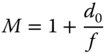
If the magnification, M, provided by the lens is defined as the ratio of the final image sizes in the two scenarios, the magnification is given by:
In describing magnifying lenses, as suggested earlier, d0 is defined to be 250 mm. Thus, a lens with a focal length of 250 mm would have a magnification of ×2 and a lens with a focal length of 50 mm would have a magnification of ×6. In practice, simple lenses are only useful up to a magnification of ×10. This is partly because of the introduction of unacceptable aberrations, but also because of the impractical short working distances introduced by lenses with a focal length of a few mm. For higher magnifications, the compound microscope must be used.
Naturally, the pupil of this simple system is defined by the pupil of the eye itself. The size of the eye's pupil varies from about 3 mm in bright light, to about 7 mm under dim lighting conditions, although this varies with individuals.
2.11.2 The Compound Microscope
In the preceding subsection, the limitations of a simple magnifying lens were made clear. Overall, its functionality, in delivering a high magnification, is to convey an intermediate image, located at the infinite conjugate, to the human eye. Furthermore, to provide maximum magnification, the focal length of this lens must be as small as possible. For practical reasons, a magnification of greater than ×10 cannot be delivered. This difficulty is solved by the compound microscope where a two-lens system is used to provide a system focal length that is considerably shorter than would be afforded by a single lens. In essence, a compound microscope consists of two lenses, or lens groups. The first lens is the objective lens that lies close to the object and the second lens, in the traditional microscope, is the eyepiece. Of course, in many modern instruments, the eye is replaced by a pixellated detector chip. Nonetheless the logic followed here still applies. Figure 2.8 shows the general set up.
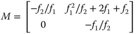
The two lenses are separated by the nominal tube length, d, and an intermediate image is formed by the objective lens within the tube. The eyepiece then presents the final image to the eye at the infinite conjugate. In other words, the intermediate image is designed to be located at a distance f2 (the eyepiece focal length) from the eyepiece. If the objective lens focal length is f1, then the matrix of the system is:

The entire co-ordinate system is referenced to the position of the objective lens. Of particular relevance here is the first focal length. From the above matrix we have the following equation for the system focal length:
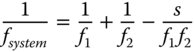
The logic of Eq. (2.9) is that a shorter system focal length can be created than would be reasonably practical with a single lens. Using the same definition as used for the simple magnifying lens, the effective system magnification, Msystem, is given by the ratio of the closest approach distance d0, (250 mm), and the system focal length. The system magnification, is given by:
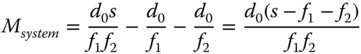
The bracketed quantity, (s − f1 − f2), i.e. the lens separation minus the sum of the lens focal lengths is known as the optical tube length of the microscope, and this will be denoted as d. Generally, for optical microscopes, this tube length is standardised across many commercial instruments with the standard values being 160 or 200 mm. Equation (2.10) may be rewritten as:
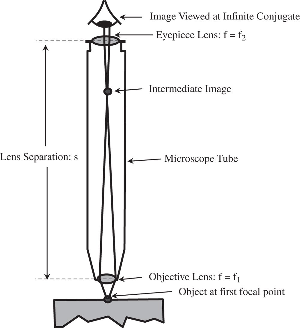
Figure 2.8 Compound microscope.
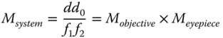
The above formula gives the total magnification of the instrument as the product of the individual magnifications of the objective lens and eyepiece. In this context, these individual magnifications are defined as in Eqs. (2.12a) and (2.12b):
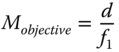
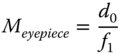
The equations above establish the standard definitions for microscope lens powers. For example, the magnification of microscope objectives is usually in the range of ×10 to ×100. For a standard tube length, d, of 160 mm, this corresponds to an objective focal length ranging from 16 to 1.6 mm. A typical eyepiece, with a magnification of ×10 has a focal length of 25 mm (d0 = 250 mm). By combining a ×100 objective lens with a ×10 eyepiece, a magnification of ×1000 can be achieved. This illustrates the power of the compound microscope.
The entrance pupil is defined by the aperture of the objective lens. This entrance pupil is re-imaged by the eyepiece to create an exit pupil that is close to the eyepiece. Ideally, this should be co-incident with the pupil of the eye. The distance of the exit pupil from final mechanical surface of the eyepiece is known as the eye relief. Placing the exit pupil further away from the physical eyepiece provides greater comfort for the user, hence the term ‘eye relief’. Objective lens aperture tends to be defined by numerical aperture, rather than f-number and range from 0.1 to 1.3 (for oil immersion microscopes).
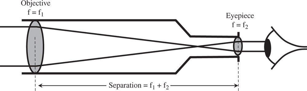
Figure 2.9 Basic optical telescope.
2.11.3 Simple Telescope
A classical optical telescope is an example of an afocal system. That is to say, no clearly defined focus is presented either in object or image space. As the name suggests, the telescope views distant objects, nominally at the infinite conjugate and provides a collimated output for ocular viewing in the case of a traditional instrument. As far as the instrument is concerned, both object and image are located at the infinite conjugate. Of course, this narrative does assume that the instrument is designed for ocular viewing as opposed to image formation at a detector or photographic plate. In any case, the design principles are similar. Fundamentally, the telescope provides angular magnification of a distant object, and this angular magnification is a key performance attribute.
The basic layout of a simple telescope is shown in Figure 2.9. Light from the distant object is collected by an objective lens whose focal length is f1 and then collimated by an eyepiece with a focal length of f2. These two lenses are separated by the sum of their focal lengths, thus creating an afocal system with an angular magnification given by the ratio of the lens focal lengths.
The matrix of the telescope is similar to that of the compound microscope, with an objective lens and eyepiece separated by some fixed distance.
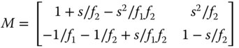
The separation, s, is simply the sum of the two focal lengths and the system matrix is given by:
The angular magnification (the D value of the matrix) is simply −f1/f2. It is important to note the sign of the magnification, so that for two positive lenses, then the magnification is negative. In line with the previous discussion with regard to the optical invariant, the linear magnification (given by matrix element A) is the inverse of the angular magnification. Also, the C element of the matrix, attesting to the focal power of the system, is actually zero and is characteristic of an afocal system.
As in the case of the microscope, the objective lens forms the system entrance pupil. The exit pupil is formed by the eyepiece imaging the objective lens. This is located a short distance, approximately f1 from the eyepiece, this distance determining the ‘eye relief’. Ideally, for ocular viewing, the pupil of the eye should be co-incident with the exit pupil. Unlike the compound microscope, the exit pupil of a simple (ocular) telescope is relatively large, about the size of the pupil of the eye. Clearly, if the exit pupil were significantly larger than the pupil of the eye, then any light falling outside the ocular pupil would be wasted. In fact, in a typical telescope, where f1 ≫ f2, the size of the exit pupil is approximately given by the diameter of the objective lens multiplied by the ratio of the focal lengths.
As an example, a small astronomical refracting telescope might comprise a 75 mm diameter objective lens with a focal length of 750 mm (f/10) and might use a ×10 eyepiece. Eyepiece magnification is classified in the same way as for microscope eyepieces and so the focal length of this eyepiece would be 25 mm, as derived from Eq. (2.12b). The angular magnification (f1/f2) would be ×30 and the size of the pupil about 3 mm, which is smaller than the pupil of the eye.
In the preceding discussion, the basic description of the instrument function assumes ocular viewing, i.e. viewing through an eyepiece. However, increasingly, across a range of optical instruments, the eye is being replaced by a detector chip. This is true of microscope, telescope, and camera instruments.
2.11.4 Camera
In essence, the function of a camera is to image an object located at the infinite conjugate and to form an image on a light sensitive planar surface. Of course, traditionally, this light sensitive surface consisted of a film or a plate upon which a silver halide emulsion had been deposited. This allowed the recording of a latent image which could be chemically developed at a later stage. Depending upon the grain size of the silver halide emulsion, feature sizes of around 10–20 μm or so could be resolved. That is to say, the ultimate system resolution is limited by the recording media as well as the optics. For the most part, this photographic film has now been superseded by pixelated silicon detectors, allowing the rapid and automatic capture and processing of images. These detectors are composed of a rectangular array of independent sensor areas (usually themselves rectangular) that each produce a charge in proportion to the amount of light collected. Resolution of these detectors is limited by the pixel size which is analogous to the grain size in photographic film. Pixel size ranges from a one micron to a few microns.
Optically from a paraxial perspective, the camera is an exceptionally simple instrument. Its purpose is simply to image light from an object located at the infinite conjugate onto the focal plane, where the sensor is located. As such, from a system perspective one might regard the camera as a single lens with the sensor located at the second focal point. This is illustrated in Figure 2.10.
If this system is the essence of simplicity, then the Pinhole Camera, a very early form of camera, takes this further by dispensing with the lens altogether! A pinhole camera relies on a very small system aperture (a pinhole) defining the image quality. In this embodiment of the camera, all rays admitted by the entrance pupil follow closely the chief ray. However, light collection efficiency is low. Whilst in the paraxial approximation, the camera presents itself as a very simple instrument, as indeed early cameras were, the demands of light collection efficiency require the use of a large aperture which results in the breakdown of the paraxial approximation. As we shall see in later chapters, this leads to the creation of significant imperfections, or aberrations, in image formation which can only be combatted by complex multi-element lens designs. Thus, in practice, a modern camera, i.e. its lens, is a relatively complex optical instrument.
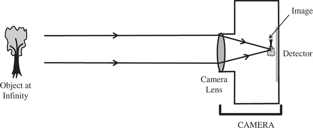
Figure 2.10 Basic camera.
In defining the function of the camera, we spoke of the imaging of an object located at infinity. In this context, ‘infinity’ means a substantially greater object distance than the lens focal length. For the traditional 35 mm format photographic camera, a typical standard lens focal length would be 50 mm. The ‘35 mm’ format refers to the film frame size which was 36 mm × 24 mm (horizontal × vertical). As mentioned in Chapter 1, the focal length of the camera lens determines the ‘plate scale’ of the detector, or the field angle subtended per unit displacement of the detector. Overall, for this example, plate scale is 1.15° mm−1. The total field covered by the frame size is ±20° (Horizontal) × ±13.5° (Vertical). ‘Wide angle’ lenses with a shorter focal length lens (e.g. 28 mm) have a larger plate scale and, naturally a wider field angle. By contrast, telephoto lenses with longer focal lengths (e.g. 200 mm), have a smaller plate scale, thus producing a greater magnification, but a smaller field of view.
Modern cameras with silicon detector technology are generally significantly more compact instruments than traditional cameras. For example, a typical digital camera lens might have a focal length of about 8 mm, whereas a mobile phone camera lens might have a focal length of about half of this. The plate scale of a digital camera is thus considerably larger than that of the traditional camera. Overall, as dictated by the imaging requirements, the field of view of a digital camera is similar to its traditional counterpart, although, in practice, equivalent to that of a wide field lens. Therefore, in view of the shorter focal length, the detector size in a digital camera is considerably smaller than that of a traditional film camera, typically a few mm. Ultimately, the miniaturisation of the digital camera is fundamentally driven by the resolution of the detector, with the pixel size of a mobile phone camera being around 1 μm. This is over an order of magnitude superior to the resolution, or ‘grain size’ of a high specification photographic film.
Further Reading
Haija, A.I., Numan, M.Z., and Freeman, W.L. (2018). Concise Optics: Concepts, Examples and Problems. Boca Raton: CRC Press. ISBN: 978-1-1381-0702-1.
Hecht, E. (2017). Optics, 5e. Harlow: Pearson Education. ISBN: 978-0-1339-7722-6.
Keating, M.P. (1988). Geometric, Physical, and Visual Optics. Boston: Butterworths. ISBN: 978-0-7506-7262-7.
Kidger, M.J. (2001). Fundamental Optical Design. Bellingham: SPIE. ISBN: 0-81943915-0.
Kloos, G. (2007). Matrix Methods for Optical Layout. Bellingham: SPIE. ISBN: 978-0-8194-6780-5.
Longhurst, R.S. (1973). Geometrical and Physical Optics, 3e. London: Longmans. ISBN: 0-582-44099-8.
Smith, F.G. and Thompson, J.H. (1989). Optics, 2e. New York: Wiley. ISBN: 0-471-91538-1.
3
Monochromatic Aberrations
3.1 Introduction
In the first two chapters, we have been primarily concerned with an idealised representation of geometrical optics involving perfect or Gaussian imaging. This treatment relies upon the paraxial approximation where all rays present a negligible angle with respect to the optical axis. In this situation, all primary optical ray behaviour, such as refraction, reflection, and beam propagation, can be represented in terms of a series of linear relationships involving ray heights and angles. The inevitable consequence of this paraxial approximation and the resultant linear algebra is apparently perfect image formation. However, for significant ray angles, this approximation breaks down and imperfect image formation, or aberration, results. That is to say, a bundle of rays emanating from a single point in object space does not uniquely converge on a single point in image space.
This chapter will focus on monochromatic aberrations only. These aberrations occur where there is departure from ideal paraxial behaviour at a single wavelength. In addition, chromatic aberration can also occur where first order paraxial properties of a system, such as focal length and cardinal point locations, vary with wavelength. This is generally caused by dispersion, or the variation in the refractive index of a material with wavelength. Chromatic aberration will be considered in the next chapter.
A simple scenario is illustrated in Figure 3.1 where a bundle of rays originating from an object located at the infinite conjugate is imaged by a lens. Figure 3.1a presents the situation for perfect imaging and Figure 3.1b illustrates the impact of aberration.
In Figure 3.1b, those rays that are close to the axis are brought to a focus at the paraxial focus. This is the ideal focus. However, those rays that are further from the axis are brought to a focus at a point closer to the lens than the paraxial focus. In fact, the behaviour illustrated in Figure 3.1b is representative of a simple lens; marginal rays are brought to a focus closer to the lens than the chief ray. However, in general terms, the sense of the aberration could be either positive or negative, with the marginal rays coming to a focus either before or after the paraxial focus.
3.2 Breakdown of the Paraxial Approximation and Third Order Aberrations
In formulating perfect or Gaussian imaging we assumed all relationships are linear. For example, Snell's law of refraction was reduced in the following way:

In making the paraxial approximation, we are considering just the first or linear term in the Taylor series. The next logical stage in the process is to consider higher order terms in the Taylor series.
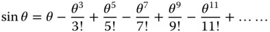
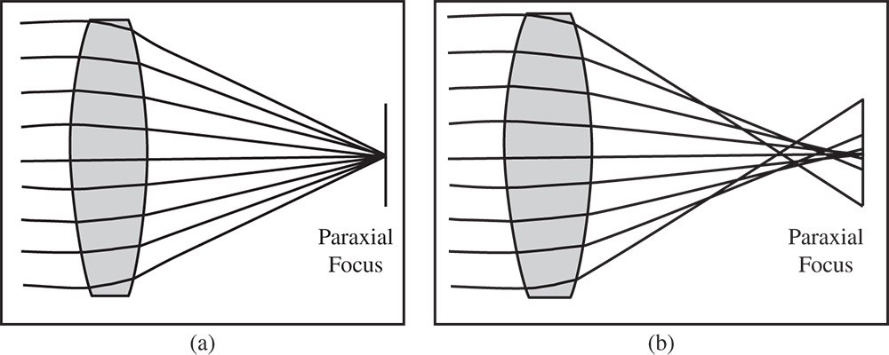
Figure 3.1 (a) Gaussian imaging. (b) Impact of aberration.
Following the term that is linear in θ, we have terms that are cubic or third order in θ. Of course, these third order terms are followed by fifth and seventh order terms etc. in succession. Third order aberration theory deals exclusively with those imperfections associated with the third order departure from ideal behaviour, as illustrated in Eq. (3.2). Much of classical aberration theory is restricted to consideration of these third order terms and is, in effect a refinement or successive approximation to paraxial theory. Higher order (≥5) terms can be important in practical design scenarios. However, these are generally dealt with by numerical computation, rather than by a simple generically applicable theory.
Third order aberration theory forms the basis of the classical treatment of monochromatic aberrations. Unless specific steps are taken to correct third order aberrations in optical systems, then third order behaviour dominates. That is to say, error terms in the ray height or angle (compared to the paraxial) have a cubic dependence upon the angle or height. As a simple illustration of this, Figure 3.1b shows rays originating from a single object (at the infinite conjugate). For perfect image formation, the height of all rays at the paraxial focus should be zero, as in Figure 3.1a. However, the consequence of third order aberration is that the ray height at the paraxial focus is proportional to the third power of the original ray height (at the lens).
In dealing with third order aberrations, the location of the entrance pupil is important. Let us assume, in the example set out in Figure 3.1b, that the pupil is at the lens. If the radius of the entrance pupil is r0 and the height a specific ray at this point is h, then we may define a new parameter, the normalised pupil co-ordinate, p, in the following way:

The normalised pupil co-ordinate can have values ranging from −1 to +1, with the extremes representing the marginal ray. The chief ray corresponds to p = 0. At this stage, it is useful to provide a specific and quantifiable definition of aberration. The quantity, transverse aberration, is defined as the difference in height of a specific ray and the corresponding chief ray as measured at the paraxial focus. The ‘corresponding chief ray’ emanates from the same object point as the ray under consideration. In addition, the term longitudinal aberration is also used to describe aberration. Longitudinal aberration (LA) is the axial distance from the point at which the ray in question intersects the chief ray and the location of the paraxial focus. The transverse aberration (TA) and longitudinal aberration definitions are illustrated in Figure 3.2.
In keeping with the previous arguments, the TA has a third order dependence upon the pupil function. This is illustrated in Eq. (3.4):

Transverse aberration has dimensions of length, whereas the pupil function is a dimensionless ratio. Geometrically, the LA is approximately equal to the transverse aberration divided by the ray angle which itself is proportional to the pupil function. Therefore, the longitudinal aberration has a quadratic dependence upon the pupil function. This is illustrated in Eq. (3.5).
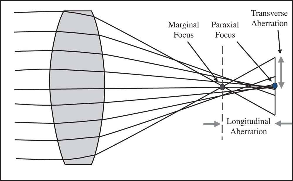
Figure 3.2 Transverse and longitudinal aberration.

In fact, if the radius of the pupil aperture is r0 and the lens focal length is f, then the longitudinal and transverse aberration are related in the following way:
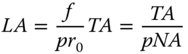
NA is the numerical aperture of the lens.
A plot of the transverse aberration against the pupil function is referred to as a ‘ray fan’. Ray fans are widely used to provide a simple description of the fidelity of optical systems. If one views the transverse aberration at the paraxial focus, then the transverse aberration should show a purely cubic dependence upon the pupil function. This is illustrated in Figure 3.3a which shows the aberrated ray fan. If, one the other hand, the transverse aberration is plotted away from the paraxial focus, then an additional linear term is present in the plot. This is because pure defocus (i.e. without third order aberration) produces a transverse aberration that is linear with respect to pupil function. This is illustrated in Figure 3.3b which shows a ray fan where both the linear defocus and third order aberration terms are present.
The underlying amount of third order aberration is the same in both plots. However, the overall transverse aberration in Figure 3.3b (plotted on the same scale) is significantly lower than that seen in Figure 3.3a. This is because defocus can, to some extent, be used to ‘balance’ the original third order aberration. As a result, by moving away from the paraxial focus, the size of the blurred spot is reduced. In fact, there is a point at which the size (root mean square radius) of the spot is minimised. This optimum focal position is referred to as the circle of least confusion. This is illustrated in Figure 3.4.
Most generally, the transverse aberration where third order aberration is combined with defocus can be represented as: