Optical Engineering Science

Smith, F.G. and Thompson, J.H. (1989). Optics, 2e. New York: Wiley. ISBN: 0-471-91538-1.

Smith, W.J. (2007). Modern Optical Engineering. Bellingham: SPIE. ISBN: 978-0-8194-7096-6.

Walker, B.H. (2009). Optical Engineering Fundamentals, 2e. Bellingham: SPIE. ISBN: 978-0-8194-7540-4.

2

Apertures Stops and Simple Instruments

2.1 Function of Apertures and Stops

In the previous chapter, we were introduced to sequential geometric optics. The simple analysis presented there is contingent upon the paraxial approximation. It is assumed that all rays in their sequential progress through the optical system always subtend a negligibly small angle with respect to the optical axis. In this scenario, the effect of all optical elements may be described in terms of a simple set of linear (in ray height and angle) equations leading to perfect image formation. This analysis, as previously outlined, is referred to as Gaussian optics.

Of course, for real, non-ideal imaging systems, the assumptions underlying the paraxial approximation break down. An inevitable consequence of this is the creation of imperfections or aberrations in the formation of images. A full treatment of these optical aberrations forms the subject of succeeding chapters. In the meantime, consideration of the paraxial approximation might suggest that these imperfections or aberrations would be enhanced for rays that make a large angle with respect to the optical axis. It seems sensible, therefore, to restrict rays emanating from an object to a specific, restricted range of angles. In practice, for most systems, this is done by inserting an opaque obstruction with a circular aperture. This circular aperture is centred on the optical axis and is known as an aperture stop and restricts rays emanating from an object. To further control scattered light, the aperture stop is usually blackened in some manner.

In addition to selecting rays close to the optical axis and thus reducing imperfections, aperture stops also control and define the amount of light entering an optical system. This will be explored in more detail in the chapters relating to radiometry or the study of the analysis and measurement of optical flux. Naturally, the larger the aperture, then the more light is passed through the system. Most usually, the system aperture is formed by a purpose made mechanical aperture that is distinct from the optical elements themselves. However, on occasion, the system aperture may be formed by the physical boundary of an optical component, such as a lens or a mirror. This is true, for example, for a reflecting or refracting telescope, where the boundary of the first, or primary mirror, forms the aperture stop.

2.2 Aperture Stops, Chief, and Marginal Rays

This principle is illustrated in Figure 2.1 which shows an object together with a corresponding aperture stop. Note that the centre of the aperture stop corresponds to the intersection of its plane with the optical axis.

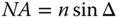
The aperture stop plays an important role in image formation and the analysis of optical systems. There are a number of important definitions relating to the aperture stop and its location. Of key significance is the chief ray which is a ray that that emanates from the object and intersects the plane of the aperture stop at its centre located at the optical axis. The angle, θ, that this ray makes with respect to the optical axis is known as the field angle. Another ray of critical importance is the marginal ray that emanates from the point where the object plane intersects the optic axis and strikes the edge of the aperture. The angle, Δ, the marginal ray makes with the axis effectively defines the size of the half angle of the cone of light emerging from a single on-axis point at the object plane and admitted by the aperture stop. The size of the aperture stop may be described either by its physical size or by the angle subtended. In the latter case, one of the most common ways of describing the aperture of an optical system is in terms of the numerical aperture (NA). The numerical aperture, is the product of the local refractive index, n, and the sine of the marginal ray angle, Δ.

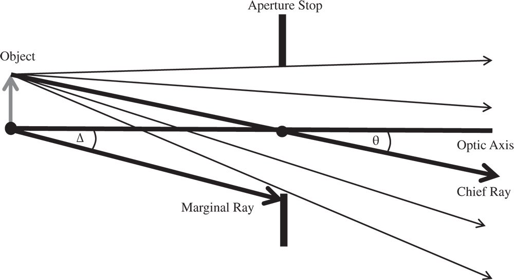
Figure 2.1 Aperture stop.

(2.1)

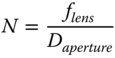
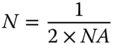
A system with a large numerical aperture, allows more light to be collected. Such a system, with a high numerical aperture is said to be ‘fast’. This terminology has its origins in photography, where the efficient collection of light using wide apertures enabled the use of short exposure times. An alternative convention exists for describing the relative size of the aperture, namely the f-number. For a lens system, the f-number, N, is given as the ratio of the lens focal length to the aperture diameter:

(2.2)

This f-number is actually written as f/N. That is to say, a lens with a focal ratio of 10 is written as f/10. The f-number has an inverse relationship to the numerical aperture and is based on the stop diameter rather than its radius. For small angles, where sinΔ = Δ, then the following relationship between the f-number and numerical aperture applies:

(2.3)

In this narrative, it is assumed that the aperture is a circular aperture, with an entire, unobstructed circular area providing access for the rays. In the majority of cases, this description is entirely accurate. However, in certain cases, this circular aperture may be partly obscured by physical or mechanical hardware supporting the optics or by holes in reflective optics. Such features are referred to as obscurations.

At this stage, it is important to emphasise the tension between fulfilment of the paraxial approximation and collection of more light. A ‘fast’ lens design naturally collects more light, but compromises the paraxial approximation and adds to the burden of complexity in lens and optical design. This inherent contradiction is explored in more detail in subsequent chapters.

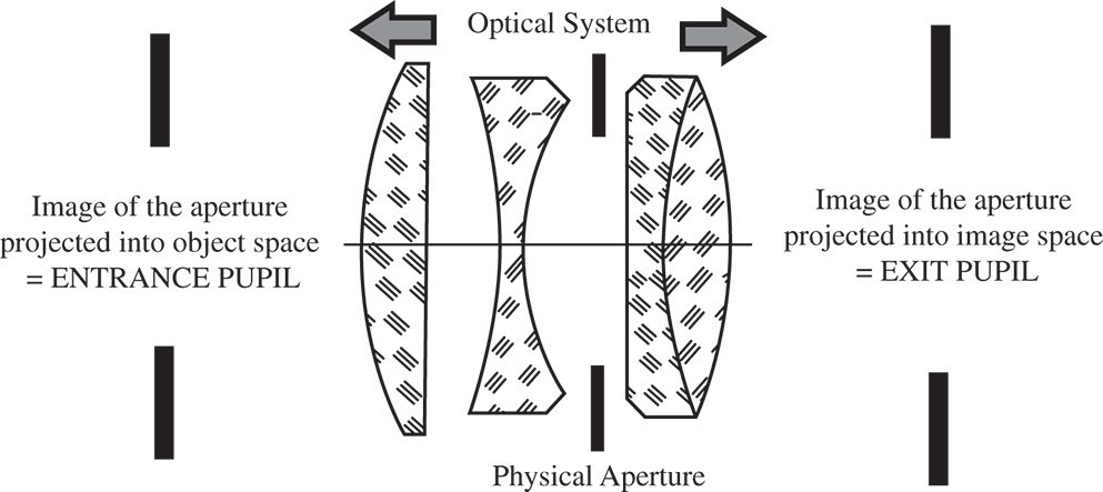
Figure 2.2 Location of entrance and exit pupils.

2.3 Entrance Pupil and Exit Pupil

The physical aperture stop may not actually be located conveniently in object space as shown in Figure 2.1. On the other hand, it may be located anywhere within the sequential train of optical components that make up the optical system. An example of this is shown in Figure 2.2, a situation that is true of many camera lenses, where the physical stop is located between lenses.

In the situation described, the entrance pupil is the image of the physical aperture as projected into object space. Correspondingly, the exit pupil is the image of the physical aperture as projected into image space. The exit pupil is located in the conjugate plane to the entrance pupil and may be regarded as the image of the entrance pupil. Along with the cardinal points of a system, the location of the entrance and exit pupils are key parameters that describe an optical system. Most particularly, the numerical aperture in object space is defined by the angle of the marginal ray that intersects the edge of the entrance pupil.

Worked Example 2.1 Cooke Triplet

Figure 2.3 shows a simplified illustration of an early type of camera lens, the Cooke triplet.

By convention, image space is assumed to be on the left-hand side of the illustration. All lenses are assumed to have no tangible thickness (thin lens approximation) and the axial origin lies at the first lens. Positive axial displacement is to the right.

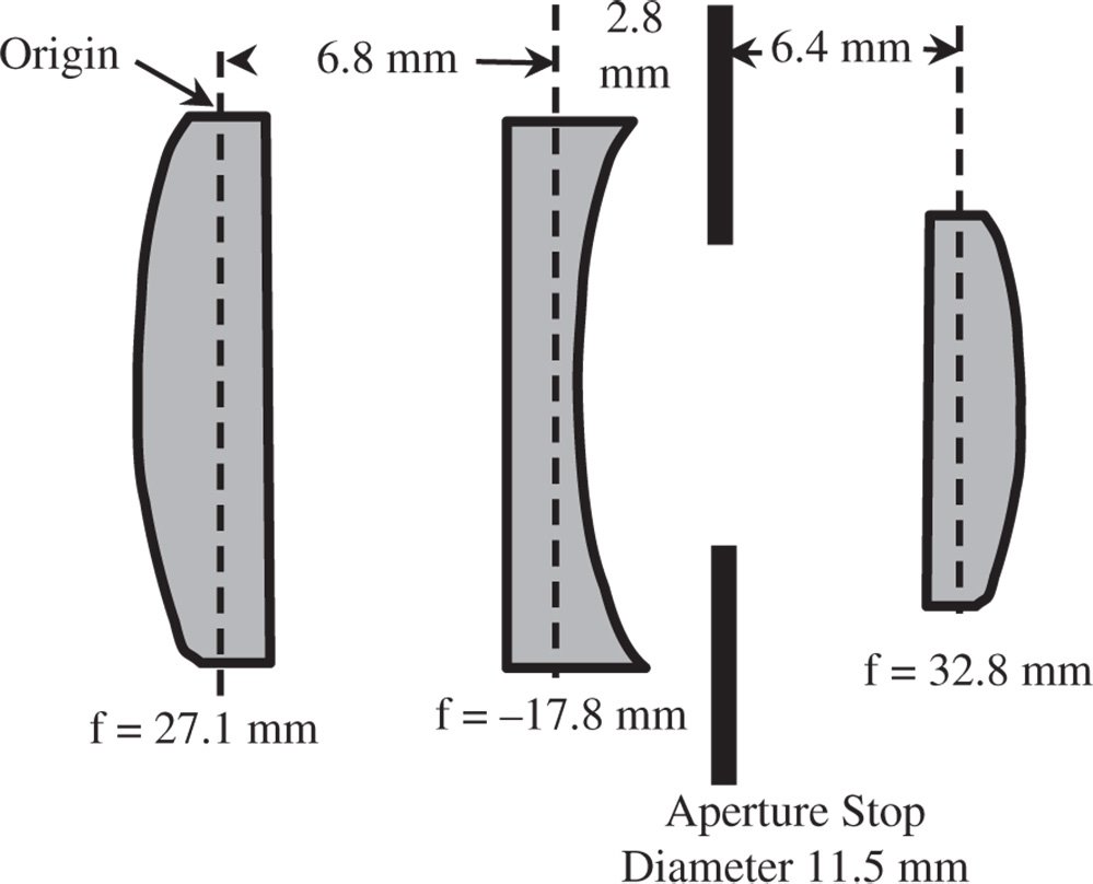
Figure 2.3 Cooke triplet.

i. Position and Size of Exit Pupil

It is easiest, first of all, to calculate the position of the exit pupil, as this is the stop imaged by a single lens (the third lens) of focal length 32.8 mm. The position of the aperture stop, the object in this instance, is 6.4 mm to the left of this lens. The distance, v, of the exit pupil from the third lens is therefore given by:

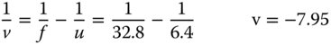
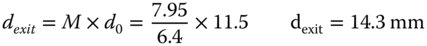
Thus, the exit pupil is 7.95 mm to the left of the third lens and 8.05 mm from the origin. The magnification is given by (minus) the ratio of image and object distances and so it is easy to calculate the size of the exit pupil:

ii. Cardinal Points of the Lens

The distance between the first and second lenses is 6.8 mm and between the second and third lenses is 9.2 mm. By convention, we retrace dummy rays −16 mm back to the origin at the first lens, so that all matrix ray tracing formulae are referred to a common origin. The matrix for the system is given below:

To calculate the position of the exit pupil we need to know the focal length of the system and the positions of the two focal points. Following the matrix relations set out in Chapter 1, we can calculate the following:

Focal length: 52.3 mm

Location of First Focal Point: −41.2 mm

Location of Second Focal Point: 57.7 mm

All distances are referenced to the axial origin at the first lens. There is, of course, a single effective focal length as both object and image spaces are considered to lie within media of the same refractive index.

iii. Position and Size of the Entrance Pupil

The imaged pupil or exit pupil lies in image space, 8.05 mm from the origin. This is 49.65 mm to the left of the second focal point. In applying Newton's formula, the second focal distance, x2 is then equal to −49.65. We can now calculate the first focal distance to determine the position of the entrance pupil.

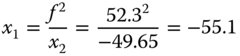
The object or entrance pupil therefore lies 55.1 mm to the right of the first focal point and 13.9 mm (−41.2 + 55.1) to the right of the first lens.

The location of the entrance pupil expressed as an object distance is 52.3 − 55.1 or −2.8 mm. Similarly the location of the exit pupil expressed as an image distance is equal to −49.65 + 52.3 or +2.65 mm. The magnification (image/object) is, in this instance equal to 2.65/2.8 or 0.946. Therefore we have:

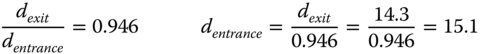
The diameter of the entrance pupil is, therefore, 15.1 mm

So, in summary we have:

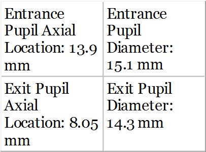
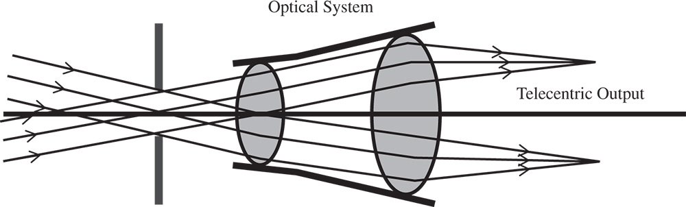
Figure 2.4 Optical system with a telecentric output.

2.4 Telecentricity

In the previous example, both entrance and exit pupils were located at finite conjugates. However, a system is said to be telecentric if the exit pupil (or entrance pupil) is located at infinity. In the case of a telecentric output, this will occur where the entrance pupil is located at the first focal point. In this instance, all chief rays will, in image space, be parallel. This is shown in Figure 2.4 which illustrates a telecentric output for two different field positions.

A telecentric output, as represented in Figure 2.4 is characterised by a number of converging ray bundles, each emanating from a specific field location, whose central or chief rays are parallel. There are a number of instances where optical systems are specifically designed to be telecentric. Telecentric lenses, for instance, have application in machine vision and metrology where non-telecentric output can lead to measurement errors for varying (object) axial positions.

2.5 Vignetting

The aperture stop is the principal means for controlling the passage of rays through an optical system. Ideally, this would be the only component that controls the admission of light to the optical system. In practice, other optical surfaces located away from the aperture stop may also have an impact on the admission of light into the system. This is because these optical components, for reasons of economy and other optical design factors, have a finite aperture. As a consequence, some rays, particularly those for larger field angles, may miss the lens or component aperture altogether. So, in this case, for field positions furthest from the optical axis, some of the rays will be clipped. This process is known as vignetting. This is shown in Figure 2.5.

Vignetting tends to darken the image for objects further away from the optical axis. As such, it is an undesirable effect. At the same time, it can be used to control optical imperfections or aberrations by deliberately removing more marginal rays.

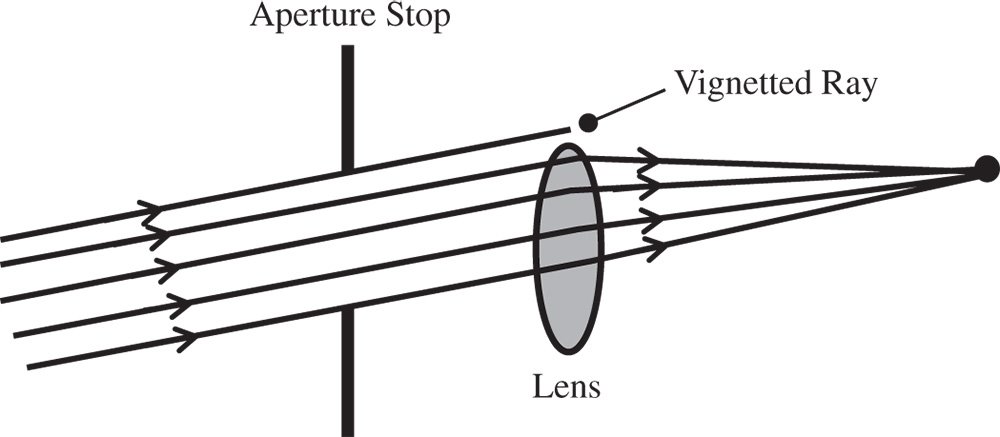
Figure 2.5 Vignetting.

2.6 Field Stops and Other Stops

In addition to the aperture stop, an optical system might also contain a field stop. This is an aperture located in a plane that is conjugate with the image plane. Its first purpose is to provide a crisp (often circular) boundary to the viewable image. Secondly, it excludes light from object locations lying outside the area of interest. In so doing, the field stop reduces the level of unwanted light that might otherwise be scattered into the image plane and so reduce image contrast. For the same reason, other, intermediate stops may be introduced into an optical design in order to further reduce the level of scattered light.

2.7 Tangential and Sagittal Ray Fans

The analysis pursued hitherto has considered the propagation of rays in a single plane. From an analytical perspective, for ray tracing in an ideal system and determining the cardinal points of that system, this is a perfectly acceptable approach. However, in reality, rays are not necessarily confined to the plane containing the object and the optical axis. With the selection of rays delineated by a two-dimensional, circular aperture, we must expect some rays to be out of this plane. A group of co-planar rays, emanating from a single object point and bounded by the entrance pupil is referred to as a ray fan. A ray fan that lies in the plane defined by the object and optical axis is known as the tangential ray fan. The sagittal ray fan emanates from the same object point and lies in a plane that is perpendicular to that of the tangential ray fan. This is illustrated in Figure 2.6.

The tangential ray fan is also referred to as the meridional ray fan; the two terms are equivalent. In general any ray that is not in the tangential plane, i.e. not a tangential ray, is referred to as a skew ray. A skew ray will never cross the optic axis.

2.8 Two Dimensional Ray Fans and Anamorphic Optics

The introduction of two distinct sets of ray fans, tangential and sagittal, together with the inclusion of skew rays confirms that sequential ray propagation in an axial geometry is essentially a two-dimensional problem. Hitherto, all discussion and, in particular, the matrix analysis, has been presented in a strictly one-dimensional form. However, the strict description of a ray in two dimensions requires the definition of four parameters, two spatial and two angular. In this more complete description, a ray vector would be written as:

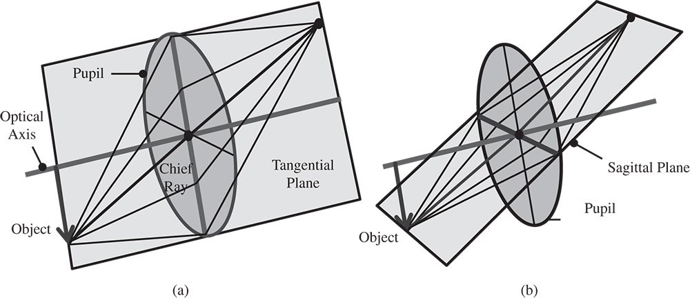
Figure 2.6 (a) Tangential ray fan; (b) Sagittal ray fan.

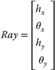
hx is the x component of the distance of the ray from the optical axis

θx is the x component of the angle of the ray to the optical axis

hy is the y component of the distance of the ray from the optical axis

θy is the y component of the angle of the ray to the optical axis

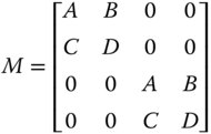
In this two dimensional representation, the matrix element representing each optical element would be a 4 × 4 matrix instead of a 2 × 2 matrix. However, the matrix is not fully populated in any realistic scenario. For a rotationally symmetric optical system, as we have been considering thus far, there can only be four elements:

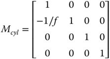
That is to say, the impact of each optical surface is identical in both the x and y directions in this instance. However, there are optical components where the behaviour is different in the x and y directions. An example of this might be a cylindrical lens, whose curvature in just one dimension produces focusing only in one direction. The two dimensional matrix for a cylindrical lens would look as follows:

A component that possesses different paraxial properties in the two dimensions is said to be anamorphic. A more general description of an anamorphic element is illustrated next:

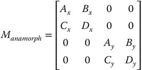
Note there are no non-zero elements connecting ray properties in different dimensions, x and y. This would require the surfaces produce some form of skew behaviour and this is not consistent with ideal paraxial behaviour. Since this is the case, the two orthogonal components, x and y, can be separated out and presented as two sets of 2 × 2 matrices and analysed as previously set out. All relevant optical properties, cardinal points are then calculated separately for x and y components. Even if focal points are identical for the two dimensions, the principal planes may not be co-located. This gives rise to different focal lengths for the x and y dimension and potentially differential image magnification. This differential magnification is referred to as anamorphic magnification. Significantly, in a system possessing anamorphic optical properties, the exit pupil may not be co-located in the two dimensions.

2.9 Optical Invariant and Lagrange Invariant

The field angle, i.e. the angle of the chief ray and the marginal ray angles, will change as the rays propagate through an optical system. The relationship between these angles is inherently constrained by the magnification properties of the optical system in the paraxial approximation. The optical invariant is a parameter that, in the paraxial approximation, constrains the relationship between any two rays that propagate through an optical system. We now have two general rays as described by their ray vectors:

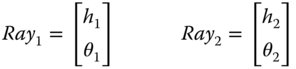
The optical invariant, O, is given by:

(2.4)

The optical invariant is, in the paraxial approximation, preserved on passage through an optical system. That is to say:

(2.5)

n′, h′, θ′, etc. are ray parameters following propagation.

Derivation of the above invariant is straightforward using matrix analysis.

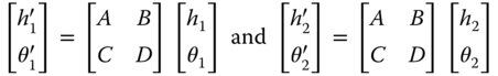
Hence:

From (1.23) we know that the determinant of the matrix is given by the ratio of the refractive indices in the relevant media, so:

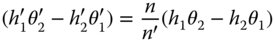
Finally we arrive at Eq. (2.5)

The optical invariant is a generalised constraint that relates system lateral and angular magnification and applies to any arbitrary pair of rays. A very specific descriptor is created when the ray pair consists of the chief ray and the marginal ray. This special case of the optical invariant is known as the Lagrange invariant. The Lagrange invariant, H is given by:

(2.6)

If we now simply evaluate H at the entrance and exit pupils where, by definition, hchief is zero, then the product nhmarginalθchief is constant. The Lagrange invariant then simply articulates the fact that the angular and lateral magnifications are inversely related. In fact, the Lagrange invariant captures a more fundamental constraint to an optical system. If the object plane is uniformly illuminated, then the total light flux emanating from the plane is proportional to the square of the maximum field angle. The proportion of that flux that is admitted by the entrance pupil is itself proportional to the square of the marginal ray height. Therefore, the total flux passing through an optical system is proportional to the square of the Lagrange invariant, H2. Thus the Lagrange invariant is an expression of the conservation of energy as light propagates through an optical system. This will become of paramount significance when, in later chapters, we consider source brightness or radiance and the impact of the optical system on optical flux flowing through it.

2.10 Eccentricity Variable

The eccentricity variable, E, is a measure of how far an axial location in an optical system is from the stop. It is expressed in terms of the chief ray to marginal ray height at that particular location. Of course, at the pupil (entrance or exit) itself, the eccentricity variable will be zero. The eccentricity variable is defined as:

(2.7)

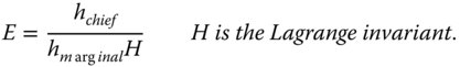
E is of course infinite at the focal point of a system. The variable is of great significance in the analysis of optical imperfections or aberrations where the distance of a component from the aperture stop is of critical importance.

2.11 Image Formation in Simple Optical Systems

These introductory chapters provide a complete description of ideal optical systems. That is to say, in the paraxial approximation, where imaging imperfections, or aberrations may be ignored, the analysis presented is substantially complete. Some very simple optical instruments are introduced at this point; their deficiencies are discussed later.

2.11.1 Magnifying Glass or Eye Loupe

The magnifying glass or eye loupe is perhaps the simplest optical system conceivable, in that is consists of a single lens that is intended to be used with the eye to magnify close objects. Our ability to resolve small, close objects is limited by our ability to focus at close quarters. Typically, although this varies with age and other factors, a comfortable distance for viewing near objects is about 250 mm. If the eye can resolve an angle of 1 arcminute, then this corresponds to a resolution of somewhat under 0.1 mm. Addition of a simple lens allows the eye to view objects at a much shorter distance. This is shown in Figure 2.7.