

Полная версия
Optical Engineering Science
1.4.4 Refraction at Two Spherical Surfaces (Lenses)
Figure 1.14 shows a lens made up of two spherical surfaces, of radius, R1 and R2. Once again, the convention is that the spherical radius is positive if the centre of curvature lies to the right of the relevant vertex.
So, in the biconvex lens illustrated in Figure 1.14, the first surface has a positive radius of curvature and the second surface has a negative radius of curvature. The lens is made from a material of refractive index n2 and is bounded by two surfaces with radius of curvature R1 and R2 respectively. It is immersed totally in a medium of refractive index, n1 (e.g. air). In addition, it is assumed that the lens has negligible thickness (the thin lens approximation). Of course, as for the treatment of the single curved surface, we assume all angles are small and θ ∼ sinθ. First, we might calculate the angle of refraction, φ1, produced by the first curved surface, R1. This can be calculated using Eq. (1.14):
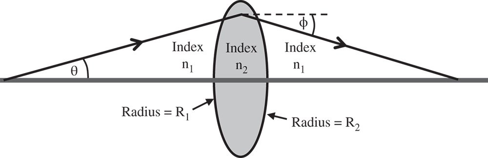
Figure 1.14 Refraction by two spherical surfaces (lens).
Of course, the final angle, φ, can be calculated from φ1 by another application of Eq. (1.14):
Substituting for φ1 we get:
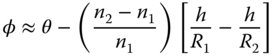
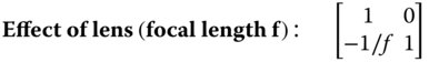
As for Eq. (1.14) there are two parts to Eq. (1.15). First, there is an angular term that is equal to the incident angle. Second, there is a focusing contribution that produces a deflection proportional to ray height. Equation (1.15) allows the tracing of all rays in a system containing the single lens and it is straightforward to calculate the Cardinal points of the thin lens: Cardinal points for a thin lens
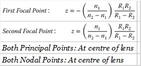
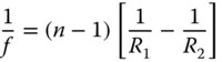
Since both object and image spaces are in the same media, then both focal lengths are equal and the principal and nodal points are co-located. One can take the above expressions for focal length and cast it in a more conventional form as a single focal length, f. This gives the so-called Lensmaker's Equation, where it is assumed that the surrounding medium (air) has a refractive index of one (i.e. n1 = 1) and we substitute n for n2.
1.4.5 Reflection by a Plane Surface
Figure 1.15 shows the process of reflection at a plane surface. As in the previous case of refraction, the reflected ray lies in the same plane as the incident ray and the angle of reflection is equal and opposite to the angle of incidence.
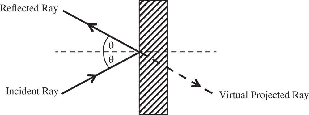
Figure 1.15 Reflection at a plane surface.
The virtual projected ray shown in Figure 1.15 illustrates an important point about reflection. If one considers the process as analogous to refraction, then a mirror behaves as a refractive material with an index of −1. This, in itself has an important consequence. The image produced is inverted in space. As such, there is no combination of positive magnification and pure rotation that will map the image onto the object. That is to say, a right handed object will be converted into a left handed image. More generally, if an optical system contains an odd number of reflective elements, the parity of the image will be reversed. So, for example, if a complex optical system were to contain nine reflective elements in the optical path, then the resultant image could not be generated from the object by rotation alone. Conversely, if the optical system were to contain an even number of reflective surfaces, then the parity between the object and image geometries would be conserved.
Another way in which a plane mirror is different from a plane refractive surface is that a plane mirror is the one (and perhaps only) example of a perfect imaging system. Regardless of any approximation with regard to small angles discussed previously, following reflection at a planar surface, all rays diverging from a single image point would, when projected as in Figure 1.15, be seen to emerge exactly from a single object point.
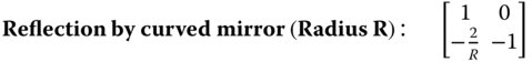
1.4.6 Reflection from a Curved (Spherical) Surface
Figure 1.16 illustrates the reflection of a ray from a curved surface.
The incident ray is at an angle, θ, with respect to the optical axis and the reflected ray is at an angle, ϕ to the optical axis. If we designate the incident angle as θ1 and the reflected angle as θ2 (with respect to the local surface normal), then the following apply, assuming all relevant angles are small:
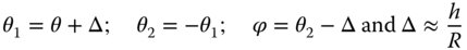
Figure 1.16 Reflection from a curved surface.
We now need to calculate the angle, ϕ, the refracted ray makes to the optical axis:
In form, Eq. (1.17) is similar to Eq. (1.14) with a linear dependence of the reflected ray angle on both incident ray angle and height. The two equations may be made to correspond exactly if we make the substitution, n1 = 1, n2 = −1. This runs in accord with the empirical observation made previously that a reflective surface acts like a medium with a refractive index of −1. Once more, the sign convention observed dictates that positive axial displacement, z, is in the direction from left to right and positive height is vertically upwards. A ray with a positive angle, θ, has a positive gradient in h with respect to z.
As with the curved refractive surface, a curved mirror is image forming. It is therefore possible to set out the Cardinal Points, as before: Cardinal points for a spherical mirror
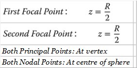
The focal length of a curved mirror is half the base radius, with both focal points co-located. In fact, the two focal lengths are of opposite sign. Again, this fits in with the notion that reflective surfaces act as media with a refractive index of −1. Both nodal points are co-located at the centre of curvature and the principal points are also co-located at the surface vertex.
1.5 Paraxial Approximation and Gaussian Optics
Earlier, in order to make our lens and mirror calculations simple and tractable, we introduced the following approximation:

That is to say, all rays make a sufficiently small angle to the optical axis to make the above approximation acceptable in practice. When this approximation is applied more generally to an entire optical system, it is referred to as the paraxial approximation (i.e. ‘almost axial’). If the same consideration is applied to ray heights as well as angles, the paraxial approximations lead to a series of equations describing the transformation of ray heights and angles that are linear in both ray height and angle. This first order theory is generally referred to as Gaussian optics, named after Carl Friedrich Gauss.
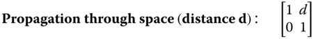
If we now assume that all rays are confined to a single plane containing the optical axis, then we can describe all rays by two parameters: θ – the angle the ray make to the optical axis and h – the height above the optical axis. If, after transformation by an optical surface, these parameters change to θ′ and h′, it is possible to write down a series of linear equations describing all transformations. These are set out in Eqs. 1.18–1.21:


Even the most complex optical system may be described as a combination of all the above elements. At first sight, therefore, it would seem that this provides a complete description of the first order behaviour of an optical system. However, there is one important, but seemingly trivial, aspect that is not considered here. This is the case of ray propagation through space. The equations are, of course simple and obvious, but we include them for completeness.

Equation (1.8) introduced the Helmholtz equation, a necessary condition for perfect image formation for an ideal system. It is clear that Gaussian optics represents a mere approximation to the ideal of the Helmholtz equation. The contradiction between the two suggests that there may be imperfections in the ideal treatment of Gaussian optics. This will be considered later when we will look at optical imperfections or aberrations. In the meantime, we will consider a very powerful realisation of Gaussian optics that takes the basic linear equations previously set out and expresses them in terms of matrix algebra. This is the so-called Matrix Ray Tracing technique.
1.6 Matrix Ray Tracing
1.6.1 General
In Section 1.4 we looked at the behaviour of some very simple components, mirrors and lenses, deriving the locations of the Cardinal Points. As discussed previously, the Cardinal Points provide a complete description of the first order properties of an optical system, no matter how complex.
The question then is how do we calculate the properties of a more complex optical system, such as the camera lens depicted in Figure 1.17? It is not immediately obvious where the Cardinal points lie or what the focal length is. However, we can combine the generalised description of an optical system with the treatment of Gaussian optics to produce a model that describes the entire system as a black box acting on rays with a simple linear transformation. The black box may be visualised as below in Figure 1.18.
Following the basic premise of Gaussian optics, we can relate the input and output rays using a set of linear equations:
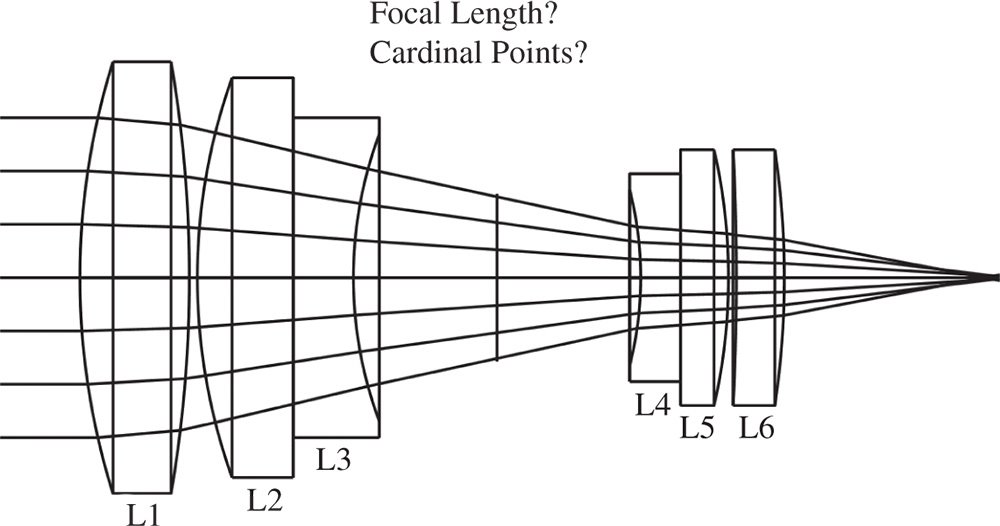
Figure 1.17 Complex optical system.
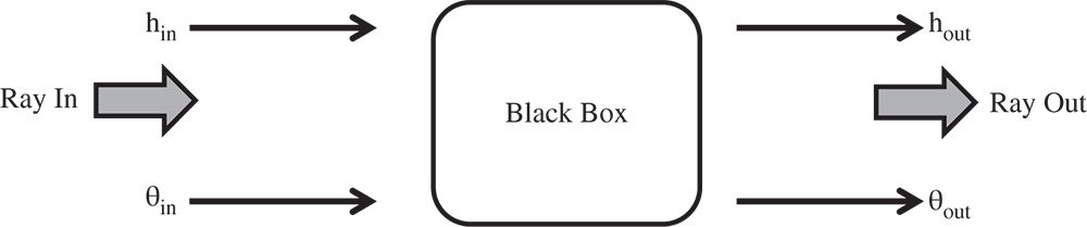
Figure 1.18 Modelling of complex systems.
Equations (1.23) and (1.24) may be combined in a matrix representation:
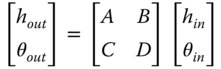
Equation (1.25) sets out the Matrix Ray Tracing convention used in this book. The reader should be aware that other conventions are used, but this is the most widely used. Equation (1.25) can be used to describe the overall system matrix or that of individual components. The question is how to build up a complex system from a large number of optical elements. The camera lens shown in Figure 1.17 has six lenses and we might represent each lens as a single matrix, i.e. M1, M2,…..,M6. Each matrix describes the relationship between rays incident upon the lens and those leaving. The impact of successive optical elements is determined by successive matrix multiplication. So the system matrix for the lens as a whole is given by the matrix product of all elements:

Note the order of the multiplication; this is important. M1 represents the first optical element seen by rays incident upon the system and the multiplication procedure then works through elements 2–6 successively. For purposes of illustration, each lens has been treated as being represented by a single matrix element. In practice, it is likely that the lens would be reduced to its basic building blocks, namely the two curved surfaces plus the propagation (thickness) between the two surfaces. We also must not forget the propagation through the air between the lens elements.
Representation of the key optical surfaces can be determined by casting Eqs. (1.18)–(1.22) in matrix format.
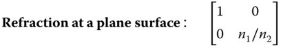
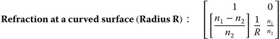
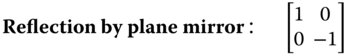
n1 and n2 represent the refractive index of first and second media respectively.
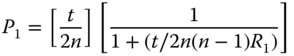
1.6.2 Determination of Cardinal Points
It is very straightforward to calculate the Cardinal Points of a system from the system matrix:

The matrix above represents the system matrix after propagating through all optical elements as shown in Figure 1.17. However, the convention adopted here is that an additional transformation is added after the final surface. This additional transformation is free space propagation to the original starting point. It must be emphasised that, this is merely a convention, and that the final step traces a dummy ray as opposed to a real ray. That is to say, in reality, the light does not propagate backwards to this point. In fact, this step is a virtual back-projection of the real ray which preserves the original ray geometry. The logic of this, as will be seen, is that in any subsequent analysis, the location of all cardinal points is referenced with respect to a common starting point. If this step were dispensed with, then the three first Cardinal Points would be referenced to the start point and the three second Cardinal Points to the end point. With this in mind, the Cardinal Points, as referenced to the common start point are set out below; the reader might wish to confirm this.
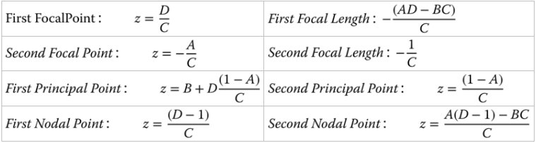
The determinant of the matrix, (AD−BC), is a key parameter. The ratio of the two focal lengths of the system is simply given by the determinant. That is to say the ratio of the two focal lengths is given by:
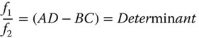
Inspecting all matrix expressions in Eqs. (1.27a–1.27f), the determinant of the matrix is simply n1/n2, the ratio of the indices in the two media, for all possible scenarios. Since the determinant of a matrix product is simply the product of the individual determinants, then the determinant of the overall system matrix is simply the ratio of the refractive indices in image and object space. Thus:

This relationship was anticipated in the more generalised discussion in 1.3.9. Looking at the relationships for the principal and nodal points, it is clear when the determinant of the system matrix is unity, i.e. object and image space indices are the same, then the principal and nodal points are co-located.
In addition to the principal and nodal points, anti-principal points and anti-nodal points are sometimes (rarely) specified. Anti-principal points are conjugate points where the magnification is −1. Similarly, anti-nodal points are conjugate points where the angular magnification is −1.
1.6.3 Worked Examples
We can now use the foregoing analysis to see how matrix ray tracing might be used in practice. Here we focus on a number of useful practical examples.
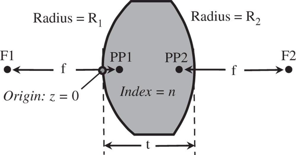
Figure 1.19 Thick lens.
Worked Example 1.1 Thick Lens
The matrix for the system is simply as below – note the order:
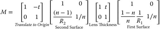
We have two translations. The first translation represents the thickness of the lens and the second translation, by convention, traces the refracted rays back to the origin in z. This is so that, in interpreting the formulae for Cardinal points, we can be sure that they are all referenced to a common origin, located as in Figure 1.19. Positive axial displacement (z) is to the right and a positive radius, R, is where the centre of curvature lies to the right of the vertex. The final matrix is as below:
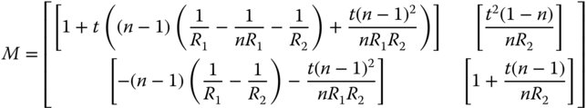
As both object and image space are in the same media, there is a common focal length, f, i.e. f1 = f2 = f. All relevant parameters are calculated from the above matrix using the formulae tabulated in Section 1.6.2.
The focal length, f, is given by:
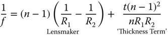
The formula above is similar to the simple, ‘Lensmaker’ formula for a thin lens. In addition there is another term, linear in thickness, t, which accounts for the lens thickness.
The focal positions are as follows:
The principal points are as follows:
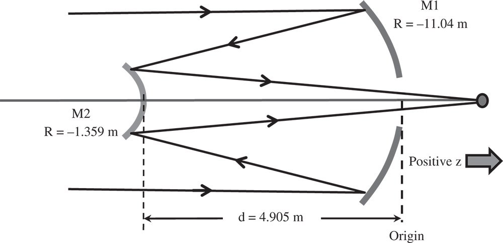
Figure 1.20 Hubble space telescope schematic.
Of course, since the refractive indices of the object and image spaces are identical, the nodal points are located in the same place as the principal points. If we take the example of a biconvex lens where R2 = −R1, then:
So, for a biconvex lens with a refractive index of 1.5, then the principal points lie about one third of the thickness from their respective vertices.
Worked Example 1.2 Hubble Space Telescope
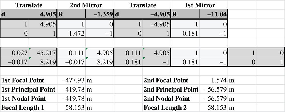
The telescope part of the Hubble Space Telescope instrument is made up of two mirrors, a primary and a secondary. Characteristics of the telescope are shown in Figure 1.20. Data is courtesy of the National Aeronautics and Space Administration.
There are four matrix elements to consider here. First, there is a mirror with a radius of −11.04 m (note sign), followed by a translation of −4.905 m (again note sign). The third matrix element is a mirror (M2) of radius − 1.359 m. Finally, we translate by +4.905 m, so that both the input and output co-ordinates are referenced with respect to the same origin. The matrices are as below:
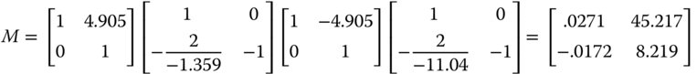
The focal positions are:

The principal points are at:

Since object and image space are in the same media, then the two focal lengths are the same. In addition, the nodal and principal points are co-located. However, when dealing with mirrors, one must be a little cautious. Each reflection is equivalent to a medium with a refractive index of −1, so that the matrix of a reflective surface will always have a determinant of −1. Therefore, any system having an even number of reflective surfaces, as in this example, then its matrix will have a determinant of 1. As such, the two focal lengths will be the same and principal and nodal points co-located. However, where there are an odd number of reflective surfaces, assuming object and image spaces are surrounded by the same media, then f2 = −f1. In this instance, principal and nodal points are separated by twice the focal length.
Although, in terms of overall length, the telescope is compact, ∼5 m primary–secondary separation, the focal length, at 58 m, is long. The focal length of the instrument is fundamental in determining the ‘plate scale’ the separation of imaged objects (stars, galaxies) at the (second) focal plane as a function of their angular separation. As such, a long focal length, of the order of 60 m, may have been a requirement at the outset. At the same time, for practical reasons, a compact design may also have been desired. One may begin to glance, therefore, at the significance, at the very outset of these very basic calculations in the design of complex optical instruments.
1.6.4 Spreadsheet Analysis
For the examples previously set out, matrix multiplication is a quick and convenient method for calculating the first order parameters of an optical system. Nonetheless, it must be recognised that as systems become more complex, with more optical surfaces, these calculations can become quite tedious. However, these matrix calculations are easy to embed with spreadsheet tools enabling the automatic computation of all cardinal points. By way of example, the previous calculation is set out and automated using a simple spreadsheet tool.
In the exercises that follow, the reader may choose to use this method to simplify calculations.
Further Reading
Born, M. and Wolf, E. (1999). Principles of Optics, 7e. Cambridge: Cambridge University Press. ISBN: 0-521-642221.
Haija, A.I., Numan, M.Z., and Freeman, W.L. (2018). Concise Optics: Concepts, Examples and Problems. Boca Raton: CRC Press. ISBN: 978-1-1381-0702-1.
Hecht, E. (2017). Optics, 5e. Harlow: Pearson Education. ISBN: 978-0-1339-7722-6.
Keating, M.P. (1988). Geometric, Physical, and Visual Optics. Boston: Butterworths. ISBN: 978-0-7506-7262-7.
Kidger, M.J. (2001). Fundamental Optical Design. Bellingham: SPIE. ISBN: 0-81943915-0.
Kloos, G. (2007). Matrix Methods for Optical Layout. Bellingham: SPIE. ISBN: 978-0-8194-6780-5.
Longhurst, R.S. (1973). Geometrical and Physical Optics, 3e. London: Longmans. ISBN: 0-582-44099-8.
Riedl, M.J. (2009). Optical Design: Applying the Fundamentals. Bellingham: SPIE. ISBN: 978-0-8194-7799-6.
Saleh, B.E.A. and Teich, M.C. (2007). Fundamentals of Photonics, 2e. New York: Wiley. ISBN: 978-0-471-35832-9.