Optical Engineering Science

c is the speed of light in vacuo and ds is an element of path between A and B

This is illustrated in Figure 1.3.

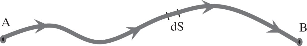
Figure 1.3 Arbitrary ray path between two points.

Fermat's principle may then be stated as follows:

Light will travel between two points A and B such that the path taken represents a local minimum in the total optical path between these points.

Fermat's principle underlies all ray optics. All laws governing refraction and reflection of rays may be derived from Fermat's principle. Most importantly, to demonstrate the theoretical foundation of ray optics and its connection with physical or wave optics, Fermat's principle may be directly derived from the wave equation. This proof demonstrates that the path taken represents, in fact, a stationary solution with respect to other possible paths. That is to say, technically, the optical path taken could represent a local maximum or inflexion point rather than a minimum. However, for most practical purposes it is correct to say that the path taken represents the minimum possible optical path.

Fermat's principle is more formally set out in the Eikonal equation. Referring to Figure 1.2, if instead of describing the light in terms of rays it is described by the wavefront surfaces themselves. The function S(r) describes the phase of the wave at any point and the Eikonal equation, which is derived from the wave equation, is set out thus:

(1.4)

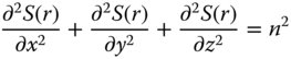
The important point about the Eikonal equation is not the equation itself, but the assumptions underlying it. Derivation of the Eikonal equation assumes that the rate of change in phase is small compared to the wavelength of light. That is to say, the radius of curvature of the wavefronts should be significantly larger than the wavelength of light. Outside this regime the assumptions underlying ray optics are not justified. This is where the effects of the wave nature of light (i.e. diffraction) must be considered and we enter the realm of physical optics. But for the time being, in the succeeding chapters we may consider that all optical systems are adequately described by geometrical optics.

So, for the purposes of this discussion, it is one simple principle, Fermat's principle, that provides the foundation for all ray optics. For the time being, we will leave behind specific consideration of the detailed behaviour of individual optical surfaces. In the meantime, we will develop a very generalised description of an idealised optical system that does not attribute specific behaviours to individual components. Later on, this ‘black box model’ will be used, in conjunction with Gaussian optics to provide a complete first order description of complex optical systems.

1.3 Sequential Geometrical Optics – A Generalised Description

In applying geometrical optics to a real system, we are attempting to determine the path of a ray(s) through the system. There are a few underlying characteristics that underpin most optical systems and help to simplify analysis. First, most optical systems are sequential. An optical system might comprise a number of different elements or surfaces, e.g. lenses, mirrors, or prisms. In a sequential optical system, the order in which light propagates through these components is unique and pre-determined. Second, in most practical systems, light is constrained with respect to a mechanical or optical axis of symmetry, the optical axis, as illustrated in Figure 1.4. In real optical systems, light is constrained by the use of physical apertures or ‘stops’; this will be discussed in more detail later.

Of course, in practice, the optical axis need not be a continuous, straight line through an optical system. It may be bent, or folded by mirrors or prisms. Nevertheless, there exists an axis throughout the system with respect to which the rays are constrained.

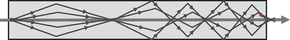
Figure 1.4 Constraint of rays with respect to optical axis.

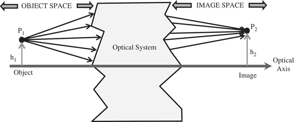
Figure 1.5 Generalised optical system and conjugate points.

1.3.1 Conjugate Points and Perfect Image Formation

We consider an ideal optical system which consists of a point source of light, the object, and an optical system that collects the light and re-directs all rays emanating from this point source or object, such that the rays converge onto a single point, the image point. At this stage, the interior workings of the optical system are undefined; the system behaves as a ‘black box’. The object is said to be located in object space and the image in image space and the pair of points are said to be conjugate points. This is illustrated in Figure 1.5.

In Figure 1.5, the two points P1 and P2 are conjugate. The optical system can be simple, for example a single lens, or it can be complex, containing many optical elements. The description above is entirely generalised. Where the object point lies on the optical axis, its image or conjugate point also lies on the optical axis. In Figure 1.5, the object point has a height of h1 with respect to the optical axis and its corresponding image point has a height of h2 with respect to the same axis. The ratio of these two heights gives the system (transverse) magnification, M:

(1.5)

Points occupying a plane perpendicular to the optical axis are conjugate to points lying on another plane perpendicular to the optical axis. These planes are known as conjugate planes.

1.3.2 Infinite Conjugate and Focal Points

Where an image or object is located at infinity, all rays emerging from or travelling to these locations will be parallel with respect to each other. In this instance, the point located at infinity is said to be at an infinite conjugate. The corresponding conjugate point to the infinite conjugate is known as a focal point. There are two focal points. The first focal point is located in the object space with the corresponding image located at the infinite conjugate. The second focal point is located in the image space with the object placed at the infinite conjugate. Figure 1.6 depicts the first focal point:

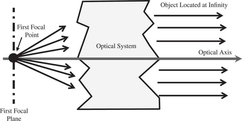
Figure 1.6 Location of first focal point.

As well as focal points, there are two corresponding focal planes. The two focal planes are planes perpendicular to the optical axis that contain the relevant focal point. For all points lying on the relevant focal plane, the conjugate point will lie at the infinite conjugate. In other words, all rays will be parallel with respect to each other. In general, the rays will not be parallel to the optic axis. This would only be the case for a conjugate point lying on the optical axis.

1.3.3 Principal Points and Planes

All points lying on a particular conjugate plane are associated with a specific transverse magnification, M, which is equal to the ratio of the image and object heights. For an ideal system, there exist two conjugate planes where the magnification is unity. These are known as the principal planes. Thus, there are two principal planes and the points where the optical axis intersects the principal planes are known as principal points. The first principal point (plane) is located in object space and the second principal point (plane) is located in image space. The arrangement is illustrated schematically in Figure 1.7.

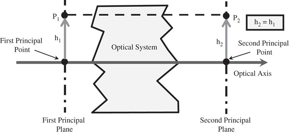
Figure 1.7 Principal points and principal planes.

1.3.4 System Focal Lengths

The reader might be used to ascribing a single focal length to an optical system, such as for a magnifying lens or a camera lens. However, in this general description, the system has two focal lengths. The first focal length, f1, is the distance from the first focal plane (or point) to the first principal plane (or point) and the second focal length, f2, is the distance from the second principal plane to the second focal plane. In many cases, f1 and f2 are identical. In fact, the ratio f1/f2 is equal to n1/n2, the ratio of the refractive indices of the media associated with the object and image spaces. However, this need not concern us at this stage, as the treatment presented here is entirely general and independent of the specific attributes of components or media.

In classical geometrical optics, the object location is denoted by the object distance, u, and the image location by the image distance, v. In the context of this general description, the object distance is simply the distance from the object to the first principal plane. Correspondingly, the image distance, v, is the distance from the second principal plane to the image. In addition, the object location can be described by the distance, x1, separating the object from the corresponding focal plane. Similarly, x2 represents the distance from the image to the second focal plane. This is illustrated in Figure 1.8.

1.3.5 Generalised Ray Tracing

This general description of an optical system is very economical in that the definition of conjugate points, focal planes, and principal planes provides sufficient information to determine the path of a ray in the image space, given the path of the ray in the object space. No assumptions are made about the internal workings of the optical system; it is merely a ‘black box’.

We see how input rays originating in the object space are mapped onto the image space for specific scenarios where the object is located at the input focal plan, the infinite conjugate, or the first principal plane. How can this be extended to determine the output path of any input ray? The general principle is set out in Figure 1.9. First, the input ray is traced from point P1 as far as its intersection with the (first) principal plane at A1. We know that this point, A1, is conjugated with point A2, lying at the same height at the second principal plane. This follows directly from the definition of principal planes. Second, we draw a dummy ray originating from the first focal point, f1, but parallel to the input ray and trace it to where it intersects the first principal plane at B1. We know that B1 is conjugated with point B2, lying at the same height on the second principal plane. Since this ray originated from the first focal point, its path must be parallel to the optical axis in image space and thus we can trace it as far as the second focal plane at P2. Finally, since the object ray and dummy rays are parallel in object space, they must meet at the second focal plane in the image space. Therefore, we can trace the image ray to point P2, providing a complete definition of the path of the ray in image space.

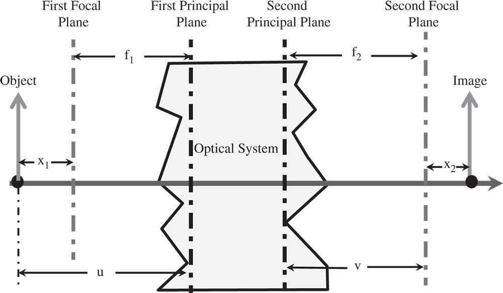
Figure 1.8 System focal lengths.

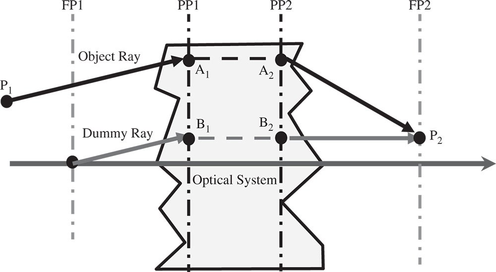
Figure 1.9 Tracing of arbitrary ray.

1.3.6 Angular Magnification and Nodal Points

The angular magnification of an optical system is the ratio of the angle (with respect to the optical axis) of a ray in image space and that of its conjugate in object space. There exists a pair of conjugate points lying on the optical axis where, for all possible rays, the angular magnification is unity. These are the nodal points. The first nodal point is located in object space and the second nodal point is located in image space. This is set out in Figure 1.10, where for a general conjugate pair, the angular magnification, α, is equal to θ2/θ1. For the nodal points, θ2 = θ1; that is to say, the angular magnification is unity. Where the two focal lengths are identical, or the object and image spaces are within media of the same refractive index, the nodal points are co-located with the principal points.

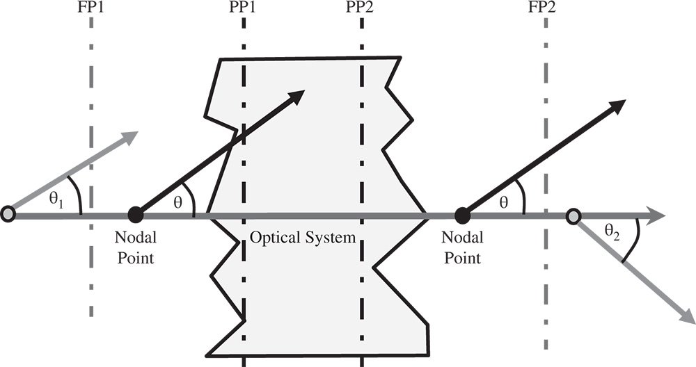
Figure 1.10 Angular magnification and nodal points.

1.3.7 Cardinal Points

This brief description has provided a complete definition of an ideal optical system. No matter how complex (or simple) the optical system, this analysis defines the complete end-to-end functionality of an ideal system. On this basis, an optical designer will specify the six cardinal points of a system to describe the ideal behaviour of a design. These six cardinal points are:

First Focal Point

Second Focal Point

First Principal Point

Second Principal Point

First Nodal Point

Second Nodal Point

The principal and nodal points are co-located if the two system focal lengths are identical.

1.3.8 Object and Image Locations – Newton's Equation

The location of the cardinal points has given us a complete description of a generalised optical system. Given that the function of an optical system might be to produce an image of an object located at a specific point, we might want to know the location of that image. Figure 1.11 shows the relationship between a generalised object and image.

Referring to Figure 1.11 and by using similar triangles it is possible to derive two separate relations for the magnification h2/h1:

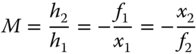
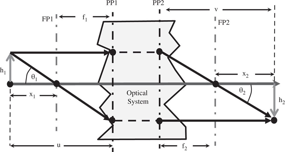
Figure 1.11 Generalised object and image.

And:

(1.6)

The above equation is Newton's Equation and may be re-cast into a more familiar form using the definitions of object and image distances, u and v, as previously set out.

(1.7)

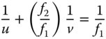
If f1 = f2 = f, we are left with the more familiar lens equation. However, Eq. (1.7) is generally applicable to all optical systems. Most importantly, Eq. (1.7) will give the locations of the object and image in systems of arbitrary complexity. Many readers might have encountered Eq. (1.7) in the context of a simple lens where object and image distances are obvious and easy to determine. For a more complex system, one has to know the location of the principal planes as well in order to determine the object and image distances.

1.3.9 Conditions for Perfect Image Formation – Helmholtz Equation

Thus far, we have presented a description of an idealised optical system. Is there a simple condition that needs to be fulfilled in order to generate such an ideal image? It is easy to see from Figure 1.11 that the following relations apply:

Therefore:

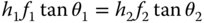
As we will be able to show later, the ratio f2/f1 is equal to the ratio of the refractive indices, n2/n1, in the two media (object and image space). Therefore it is possible to cast the above equation in its more usual form, the Helmholtz equation:

(1.8)

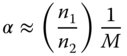
One important consequence of the Helmholtz equation is that there is a clear, inextricable linkage between transverse and angular magnification. Angular magnification is inversely proportional to transverse magnification. For small θ, tan θ and θ are approximately equal. So in the small signal approximation, the angular magnification, α is given by:

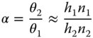
Hence:

(1.9)

We have, thus far, introduced two different types of optical magnification – transverse and angular. There is a third type of magnification that we need to consider, longitudinal magnification. Longitudinal magnitude, L, is defined as the shift in the axial image position for a unit shift in the object position, i.e.:

(1.10)

From Newton's Eq. (1.6):

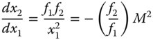
And:

(1.11)

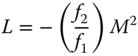
Thus, the longitudinal magnification is proportional to the square of the transverse magnification.

1.4 Behaviour of Simple Optical Components and Surfaces

1.4.1 General

The analysis presented thus far is entirely independent of the optical components that might populate the idealised optical system. In this section we will begin to consider, from the perspective of ray optics, the behaviour of real elements that make up this generalised system. At a basic level, only a few behaviours need to be considered in order to understand the propagation of rays through a real optical system. These are:

Propagation through a homogeneous medium

Refraction at a planar surface

Refraction at a curved (spherical) surface

Refraction through lenses

Reflection at a planar surface

Reflection at a curved (spherical) surface

As previously set out, the path of rays through a system is governed entirely by Fermat's principle. From this point, we will apply the simplest definition of Fermat's principle and assume that the time or optical path of rays is minimised. As far as propagation through a homogeneous medium is concerned, this leads to a perhaps obvious and trivial conclusion that light travels in straight lines. In fact, this describes a specific application of Fermat's principal, known as Hero's principle, namely that light follows the path of minimum distance between two points within a homogeneous medium.

1.4.2 Refraction at a Plane Surface and Snell's Law

The law governing refraction at a planar surface is universally attributed to Willebrord Snellius and referred to as Snell's law. This states that both incident and refracted rays lie in the same plane and their angles of incidence and refraction (with respect to surface normal) are given by:

(1.12)

This is illustrated in Figure 1.12.

The refractive indices of some optical materials (at 550 nm) are listed below:

Glass (BK7): 1.52

Plastic (Acrylic): 1.48

Water: 1.33

Air: 1.00027

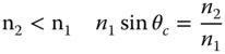
Snell's law is, in fact, a direct consequence of Fermat's principle. The reader may wish to derive this through the application of differential calculus. In finding the optimum path from a point in one medium to a point in another medium, the ray will attempt, as far as possible, to minimise its path through the higher index medium. Snell's law thus represents the minimum optical path condition in this instance. Where the ray passes from a high index material to a low index material, there exists an angle of incidence where the angle of refraction is 90°. This angle is known as the critical angle and, for angles of incidence beyond this, the ray is totally internally reflected. The critical angle, θc, is given by:

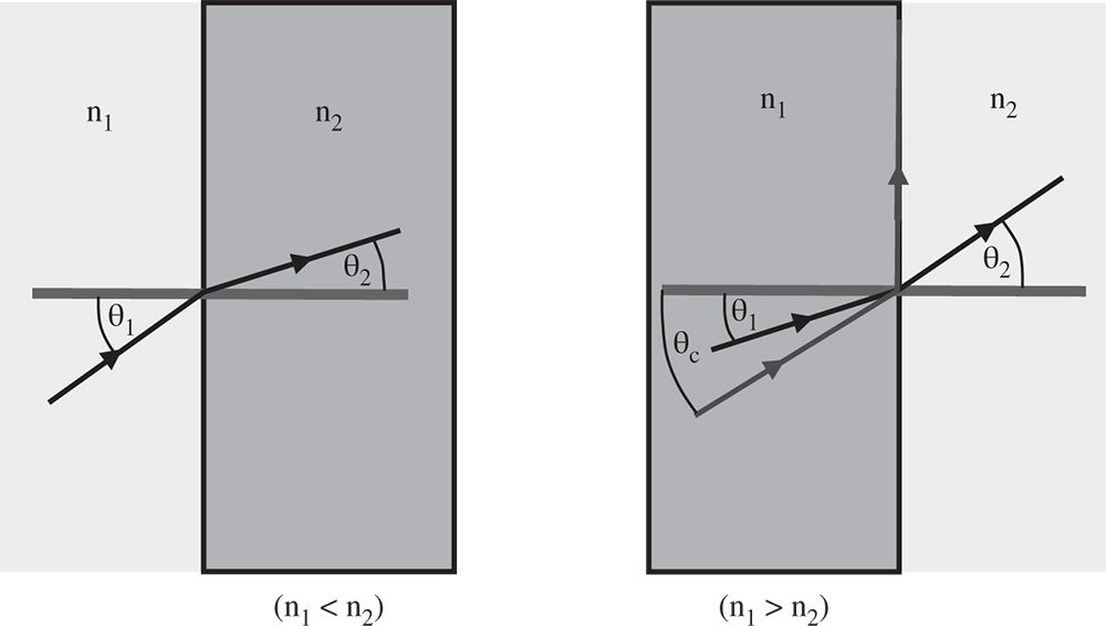
Figure 1.12 Refraction at a plane surface.

(1.13)

A single refractive surface is an example of an afocal system, where both focal lengths are infinite. Although it does not bring a parallel beam of light to a focus, it does form an image that is a geometrically true representation of the object.

1.4.3 Refraction at a Curved (Spherical) Surface

Most, if not all, curved optical surfaces are at least approximately spherical and are widely employed in the fabrication of lens components. Figure 1.13 illustrates refraction at a spherical surface.

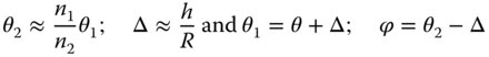
As before, the special case of refraction at a spherical surface may be described by Snell's law:

If we now wish to calculate the angle φ in terms of θ, this process is, in principle, straightforward. We need also to take into account the angle the surface normal makes with the optical axis, Δ, and the radius of curvature, R, of the spherical surface. However, calculation is a little unwieldy, so therefore we make the simplifying assumption that all angles are small and:

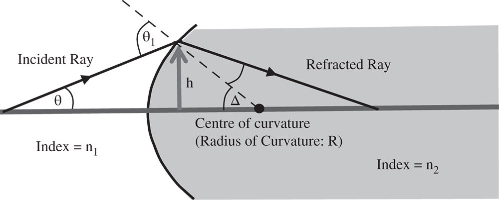
Figure 1.13 Refraction at a spherical surface.

Hence:

We can finally calculate φ in terms of θ:

(1.14)

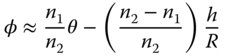
There are two terms on the RHS of Eq. (1.14). The first term, depending on the input angle θ is of the same form as Snell's law (for small angles) for a plane surface. The second term, which gives an angular deflection proportional to the height, h, and inversely proportional to the radius of curvature R, provides a focusing effect. That is to say, rays further from the optic axis are bent inward to a greater extent and have a tendency to converge on a common point. The sign convention used here assumes that positive height is vertically upward, as displayed in Figure 1.13 and a positive spherical radius corresponds to a scenario in which the centre of the sphere lies to the right of the point where the surface intersects the optical axis. Finally, a positive angle is consistent with an increase in ray height as it propagates from left to right in (1.13).

Equation (1.14) can be used to trace any ray that is incident upon a spherical refractive surface. If this surface is deemed to comprise ‘the optical system’ in its entirety, then one can use Eq. (1.14) to calculate the location of all Cardinal Points, expressed as a displacement, z along the optical axis. Positive z is to the right and the origin lies at the intersection of the optical axis and the surface. The Cardinal points are listed below. Cardinal points for a spherical refractive surface

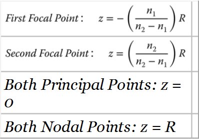
In this instance, the two focal lengths, f1 and f2 are different since the object and image spaces are in different media. If we take the first focal length as the distance from the first focal point to the first principal point, then the first focal length is positive. Similarly, the second focal length, the distance from the second principal point to the second focal point, is also positive. The principal points are both located at the surface vertex and the nodal points at the centre of curvature of the sphere. It is important to note that, in this instance, the principal and nodal points do not coincide. Again, this is because the refractive indices of object and image space differ.