Полная версия
Optical Engineering Science
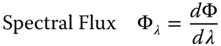
We can now illustrate this process by considering a slit with a width of 2 mm which is illuminated by a 500 nm source. By reference to the example of Gaussian beam propagation, we assume in this analysis that the illumination is significantly spatially coherent. This does not necessarily imply the use of a laser beam; in practice it means that the slit is illuminated by a parallel beam with very small angular divergence. We now view the slit at a distance of 100 mm. The Fresnel number is 20 and, as the effective angle, θ, is 0.01 rad, the Fresnel approximation is clearly justified by applying Eq. (6.50). Applying the Fresnel integral to this specific problem, we obtain the flux distribution described by Figure 6.16.
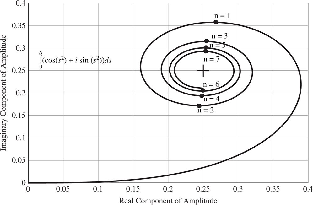
Figure 6.15 Fresnel integral and Cornu spiral.
As previously indicated, the illuminated portion is described a series of fringes characterised by the spacing of the Fresnel zones. In the obscured region, the flux tails off to zero. At the slit boundary, the flux is one half of the nominal. Of course, if the set up were reversed, and an obscuration substituted for the slit, then the pattern in Figure 6.16 would be reversed.
Generally, in problems associated with Fresnel diffraction, the diffraction pattern produced by sharp edges broadly follows that illustrated in Figure 6.16. The characteristic diffraction pattern away from the sharp edge feature consists of a series of ripples denominated by the relevant Fresnel zone.
6.9 Diffraction and Image Quality
6.9.1 Introduction
The analysis of image quality is central to any analysis of an imaging system. Where the wavefront error of a system is rather larger than the operating wavelengths of the system, the performance of the system may be adequately described by geometrical optics. Metrics such as geometrical spot size, as derived directly from ray tracing, prevail in this instance. However, where the wavefront errors are very much less than this, then diffraction effects prevail. Indeed, where effects other than diffraction may be legitimately ignored, the image is said to be diffraction limited. Overall, there are a number of metrics that quantitatively describe image quality and these are summarised below:
● Geometric spot size (rms spot size, 90% encircled energy etc.) – Geometric optics
● Point spread function (rms spot size, 90% encircled energy etc.) – Wave optics
● Strehl Ratio – Wave optics
● Modulation Transfer Function (MTF)
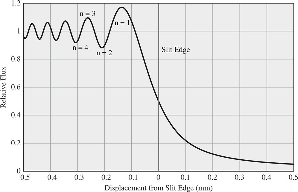
Figure 6.16 Fresnel diffraction at 100 mm from 2 mm Slit – λ = 500 nm.
6.9.2 Geometric Spot Size
This is perhaps the most straightforward of the image quality metrics to visualise. By virtue of ray tracing, for example, using ray tracing software, a number of representative rays that uniformly illuminate the entrance pupil are traced to the image plane. Of course, in an ideal image formation system, all rays would be traced to a common image point. However, deviation from this ideal behaviour is a measure of the image quality. Furthermore, this process would be attempted for a number of different field positions and, inevitably, for a dispersive system, for a number of different wavelengths. An example geometric spot is shown in Figure 6.17, illustrating the impact of spherical aberration and coma.
In order to quantify the data depicted in Figure 6.17, a number of different measures may be adopted. Measurements are characterised typically with respect to some central location. This central location may either be the intersection of the chief ray at the image plane or the weighted mean location of all intersecting rays – the centroid. That the two conventions might produce different answers is evident from the depiction of the comatic spot diagram in Figure 6.17, where the chief ray intersection corresponds to the apex at the bottom of the spot. Whichever convention is used, the size of the spot may be described in the following ways:
Figure 6.17 Geometric spots for spherical aberration and coma.
● Full width half maximum (FWHM) – the physical width in one dimension at which the flux density falls to half of the maximum
● Root mean square (rms) spot size
● Encircled energy – the physical radius within which some fixed proportion (e.g. 50% or 80%) of all rays lie.
● Ensquared energy – the size of the square within which some fixed proportion (e.g. 50% or 80%) of all rays lie
● Enslitted energy – the width of the slit within which some fixed proportion (e.g. 50% or 80%) of all rays lie
The FWHM is a useful description of the width of a sharp geometrical peak. On the other hand, the rms spot size is more mathematically useful, but not always universally applicable. In the case of an Airy disc, the rms spot size is actually infinite and the rms spot size is not so useful in situations where an image is attended by a large background signal. Encircled energy is useful to gauge the amount of light passing through a small circular aperture. Its equivalent for a rectangular geometry, the ensquared energy, is particularly useful for pixelated detectors whose sensor elements are naturally either square or rectangular. Similarly, for slitted instruments, such as spectrometers, enslitted energy is a useful metric.
Where the overall wavefront error is significantly larger than the wavelength, this geometric description of image quality is perfectly adequate. However, where this is not the case, we must look to a new approach.
6.9.3 Diffraction and Image Quality
In Section 6.5 we examined briefly the diffraction pattern produced by a uniformly illuminated pupil. This is the so-called Airy disc. The Airy disc is the diffraction pattern that one would obtain in the absence of any system aberration. In Section 6.6, we included the effect of system aberration, introducing the Huygens point spread function. The Huygens point spread function is the flux distribution pattern produced at the image plane produced by a point source at the object plane. Figure 6.18 shows an example of an aberrated pupil, where the OPD is mapped in two dimensions across a circular pupil.
The Huygens point spread function (PSF) of the same system is shown in Figure 6.19.
The PSF shown in Figure 6.19 shows much deeper rippling when compared to the Airy distribution and, unlike the geometrical analysis, represents an accurate solution for the local flux distribution at the image. In analysing the PSF, one can use similar metrics as for the geometric spot size, with the addition of the Strehl ratio:
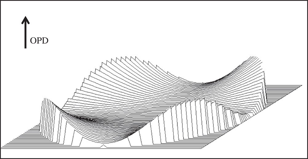
Figure 6.18 OPD map across pupil.
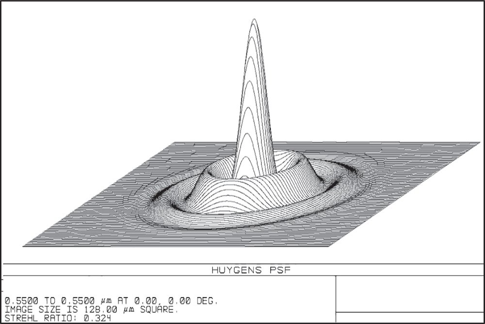
Figure 6.19 Huygens point spread function.
● Strehl Ratio
● Full width half maximum
● Root mean square (rms) spot size
● Encircled energy
● Ensquared energy
● Enslitted energy
As mentioned previously, the Strehl ratio describes the ratio of the aberrated peak flux to the unaberrated peak flux. A ratio of 0.8 or greater, by virtue of the Maréchal criterion, is considered to be ‘diffraction limited’. This is consistent with an rms wavefront error of lambda/14 or a peak to valley wavefront error of lambda/4. This measure was introduced earlier in Section 6.6, and is an exceptionally important metric to keep in mind when designing a system that is diffraction limited or near diffraction limited.
6.9.4 Modulation Transfer Function
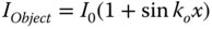
The MTF expresses the ability of an imaging system to replicate the contrast of a specific object pattern. In the case of the MTF, the object is represented by a sinusoidally varying pattern of light and dark, described by some kind of spatial frequency, ko. That is to say, the spatial variation of the object illumination is represented by:
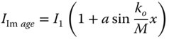
The contrast ratio of the illumination is defined as the ratio of the difference of the maximum and minimum fluxes to the sum of those fluxes. The illumination pattern represented in Eq. (6.58) has a contrast ratio of unity, with the minimum flux being zero. However, because of imaging imperfections, this is not fully represented at the image plane and the contrast is somewhat reduced. Assuming the system magnification is M, then
For an input contrast ratio of unity, the MTF is defined as the contrast ratio of the image:
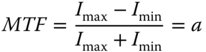
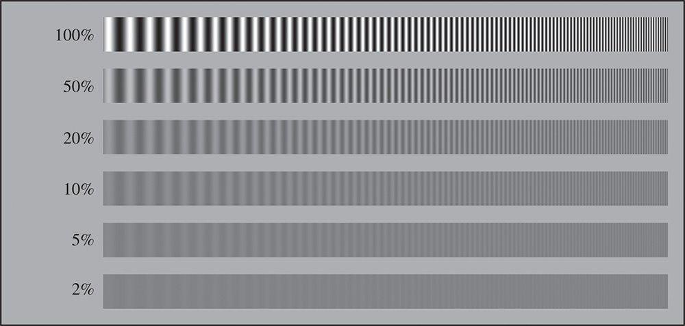
Figure 6.20 MTF pattern.
A typical example of an MTF pattern is shown in Figure 6.20.
The MTF response shown in Figure 6.20 illustrates different final contrast levels, varying from 2% to 100%. In addition, a range of input spatial frequencies is shown. In practice, there is a tendency for the contrast ratio to reduce at higher spatial frequencies; a typical imaging system has a reduced capacity for replicating fine details. A typical MTF plot against spatial frequency is shown in Figure 6.21.
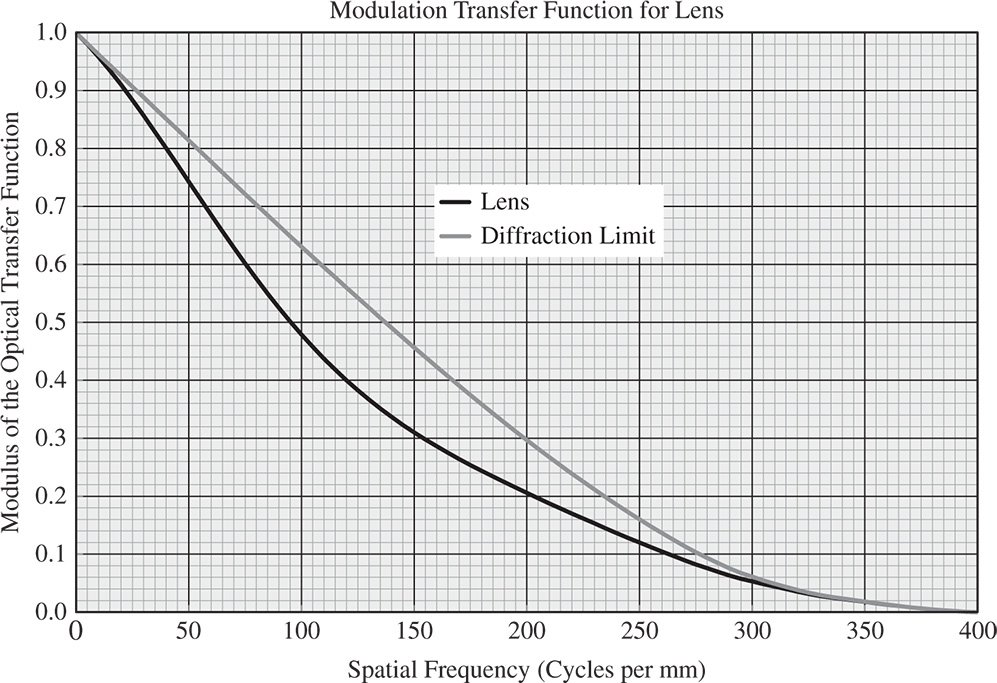
Figure 6.21 Typical MTF plot.
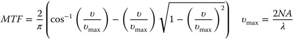
It is evident, from Figure 6.21, that the MTF declines with spatial frequency. Also included in the plot is the MTF of the diffraction limited system. In fact, the MTF is the absolute value of the complex optical transfer function (OTF). The OTF of a system is related to the Fourier transform of the point spread function. In fact, for the diffraction limited system, the MTF follows a fairly simple mathematical prescription. There is some maximum spatial frequency, υmax, above which the MTF is zero and this is defined by the system numerical aperture, NA. In this case, the diffraction limited MTF is simply given by:
The MTF is widely used in the testing and analysis of camera systems. One particular attribute of the MTF is especially useful. For a system composed of a number of subsystems, the MTF of the system is simply given by the product of the individual MTFs:

Analysis of the MTF is also useful in incorporating the behaviour of the detector. In a traditional context, where photographic film had been used, the contrast provided by the film media would be defined by the spatial frequency at which its effective MTF fell to 50%. For high contrast black and white film, this spatial frequency might have been of the order of 100 cycles per mm, although this would vary with film type and sensitivity. On the whole, colour film had poorer contrast with the equivalent spatial frequency being less than 50 cycles per mm. Of course, modern cameras base their detection upon pixelated sensors. In this instance, the characteristic spatial frequency is defined by Nyquist sampling where the equivalent spatial frequency covers two whole pixels. That is to say, for a pixel spacing of 5 μm, the equivalent spatial frequency is 100 cycles per mm.
Worked Example 6.6 We are designing a camera system to give an MTF of 0.5 at 100 cycles per mm. The camera has a pixelated detector with a pixel spacing of 5 μm. It may be assumed that the effective MTF of this detector is 0.75. The remainder of the system may be assumed to be diffraction limited. For a working wavelength of 500 nm, what is the minimum numerical aperture that the system needs to have to fulfil its requirement?
From Eq. (6.62) – the MTF of the remainder of the system is equal to 0.5/0.75 = 0.67.
Using this MTF figure we can calculate υ/υmax from Eq. (6.61) and this amounts to 0.265, giving υmax as 377 cycles per mm. Again from Eq. (6.61), given a wavelength of 500 nm, we can calculate the minimum numerical aperture of the system as 0.095 or about f#5.
6.9.5 Other Imaging Tests
The MTF provides a clearly mathematically defined test pattern for testing and subsequent analysis. However, there are other image resolution tests based upon the replication of reticulated patterns, often consisting of sharply delineated features, such as lines or line pairs. One example of this is the 1951 USAF resolution test chart which is a standard reticle placed at the object location. Broadly speaking, this consists of a set of line features whose characteristic size reduces by the sixth root of two when progressing from feature to feature. Visual inspection of the final image enables determination of the minimum line spacing resolution. The standard USAF pattern is illustrated in Figure 6.22.
Although, these types of test are inherently simpler and less capital intensive, the reliance on human visual inspection is, in itself, a weakness. Where, at one time, analytical complexity precluded the widespread use of MTF and other more abstruse processes, the availability of high performance computational power overcomes this obstacle nowadays.
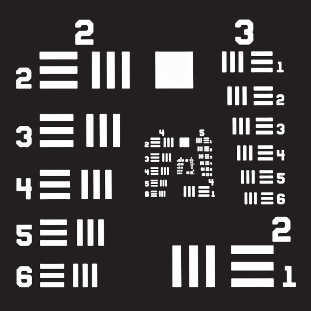
Figure 6.22 1951 USAF resolution test chart.
Source: Image Provided by Thorlabs Inc.
Further Reading
Bleaney, B.I. and Bleaney, B. (1976). Electricity and Magnetism, 3e. Oxford: Oxford University Press. ISBN: 978-0-198-51141-0.
Born, M. and Wolf, E. (1999). Principles of Optics, 7e. Cambridge: Cambridge University Press. ISBN: 0-521-642221.
Lipson, A., Lipson, S.G., and Lipson, H. (2011). Optical Physics. Cambridge: Cambridge University Press. ISBN: 978-0-521-49345-1.
Saleh, B.E.A. and Teich, M.C. (2007). Fundamentals of Photonics, 2e. New York: Wiley. ISBN: 978-0-471-35832-9.
Wolf, E. (2007). Introduction to the Theory of Coherence and Polarisation of Light. Cambridge: Cambridge University Press. ISBN: 978-0-521-82211-4.
Yariv, A. (1989). Quantum Electronics, 3e. New York: Wiley. ISBN: 978-0-471-60997-1.
7
Radiometry and Photometry
7.1 Introduction
In the preceding chapters, we have been concerned with the general behaviour of light in an optical system, as described by ray and wave propagation. Hitherto, there has been no interest in the absolute magnitude of the wave disturbance. On the other hand, radiometry and photometry is intimately concerned with the absolute flux of light within a system, its analysis and, above all, its measurement.
At this point we will make a distinction between the two terms, radiometry and photometry. Radiometry relates to analysis of the absolute magnitude of optical flux, as defined by the relevant SI unit, e.g. Watts or Watts per square metre. In contrast, photometry is concerned with the measurement of flux as mediated by the sensitivity of some detector. Most notably, although not exclusively, the detector in question might be the human eye. So, from a radiometric perspective 1 W of ultraviolet or infrared emission is worth 1 W of visible emission. However, from a photometric view (as referenced to the human eye) the ultraviolet and infrared emissions are worthless.
In the study of radiometry, we are interested in the emission of light from a physical source that might have some area dS and subtend some solid angle, dΩ. The light may either be directly emitted from a luminous source, such as a lamp filament, or scattered indirectly. The generic geometry for this is illustrated in Figure 7.1.
The geometry above may be applied both to the emission of light from a surface or to the absorption/scattering of light at a surface. The distinction between these two scenarios simply implies a reversal of the direction of travel of the rays.
7.2 Radiometry
7.2.1 Radiometric Units
For the purposes of this introduction, we will confine the initial discussion to radiometry, as opposed to photometry, where we are able to quantify the optical power of a source simply in terms of its output in watts. Fundamental to the analysis of radiometry are the radiometric quantities and their associated radiometric units. The most basic measure of an optical source is its radiant flux, Φ, measured in watts. Associated with the radiant flux is the radiant flux density, E. This refers to the total flux per unit area that is incident upon or is leaving a surface element and is measured in watts per square metre. If the radiant flux is incident upon a surface, then the radiant flux density is more usually referred to as the irradiance. If, on the other hand, the flux is emitted from the surface, it is referred to as exitance. It is of the utmost importance to apprehend that according to the strict definitions of radiometry, flux per unit area is never described as intensity. There is often a ‘colloquial’ tendency to describe flux per unit as intensity. However, this term is reserved rather for flux per unit solid angle. As such, the radiant intensity of a (point) source, I, is defined as its flux per unit solid angle and is measured in watts per steradian.
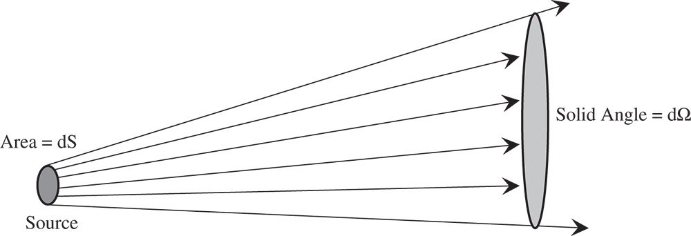
Figure 7.1 Emission from a generic source.
Table 7.1 Radiometric units.
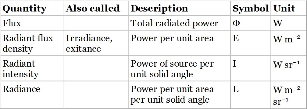
Radiance, L, is the flux arriving at or leaving a surface associated with a pencil of rays, per unit solid angle per unit surface area projected onto a plane normal to the direction of travel of those rays. It is measured in watts per square metre per steradian. Radiance is intimately related to ‘how bright’ an extended object appears and is not affected by distance from the object. For example, in the case of the sun, as one moves away from the sun, the irradiance of the solar illumination inevitably diminishes. However, the angle subtended by the solar disc reduces proportionally and the smaller solar disc would appear just as bright if one were so ill advised as to view it.
All the radiometric quantities and associated units are summarised in Table 7.1.
7.2.2 Significance of Radiometric Units
The radiant flux density can be taken as the differential of the flux with respect to area. Expressing this mathematically:

The important point to recognise about Eq. (7.1), is that the area, dS, is not only described by a scalar area, but also by a vector that defines the surface normal. Thus, orientation of the surface is of importance, and this will be described in more detail presently. Radiant intensity, may also be expressed mathematically, in this case as the differential of the flux with respect to the solid angle.

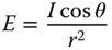
Most usually, intensity is used to describe the output of a point source. Simple geometry may be used to establish the relationship between the intensity of a point source and the irradiance it produces at a surface located at some distance from the source. This gives rise to the so-called inverse square law. The inverse square law states that the irradiance delivered by a point source to a distant object is inversely proportional to the square of the separation. Operation of the inverse square law is illustrated in Figure 7.2.
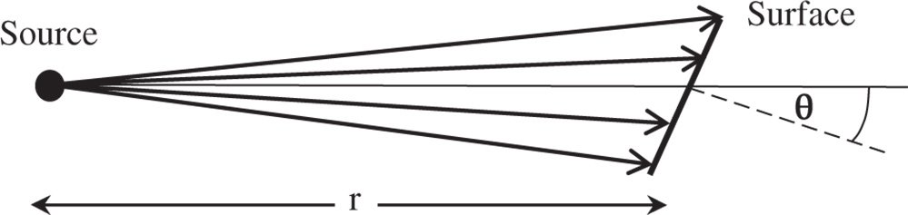
Figure 7.2 Operation of the inverse square law.
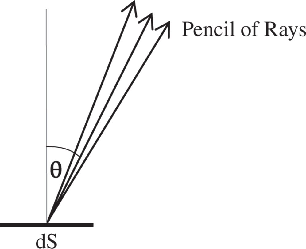
Figure 7.3 Radiance and exitance from a surface.
In the geometry illustrated in Figure 7.2, the irradiated surface is situated at a distance r from the source and its normal is at an angle θ with respect to the line joining the source at the surface. As alluded to earlier, the orientation of the surface is of some relevance. Assuming that the radiant intensity of the source is I, then the irradiance at the surface is given by:
Radiance is the flux arriving at a surface or leaving a surface per unit area, per unit solid angle. The area, in this case, is the projected area whose normal is aligned with the ray pencil, rather than the surface normal. This is illustrated schematically in Figure 7.3.
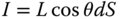
Expressing the intensity in terms of the area of an element of surface, dS, we obtain the following:
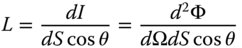
L is the radiance and I the radiant intensity.
7.2.3 Ideal or Lambertian Scattering
An ideal or Lambertian scatterer scatters light from a surface with uniform radiance irrespective of the scattering angle, θ. An imperfect approximation to a Lambertian surface might be a blank sheet of paper or a matt surface, such as a painted wall. In practice, for most surfaces, the radiance has a tendency to decline with θ. However, for a Lambertian surface, the radiant intensity of the scattered light is (from Eq. [7.4]) given by:
Hence for a Lambertian scatterer, the radiant intensity emitted from a surface element is proportional to the cosine of the angle with respect to the surface normal. In many instances, we are interested in the total amount of light scattered from a surface. This is the total hemispherical scatter or total hemispherical exitance from a surface. At first sight, this would seem to amount to the product of the solid angle, 2π, and the radiance, L. However, the radiant intensity declines according to the cosine law Eq. (7.5) and the total hemispherical exitance may be derived from the following integral, based on spherical polar co-ordinates:
Hence, the total hemispherical exitance is half what would be expected if the radiant intensity were constant as a function of polar angle.
7.2.4 Spectral Radiometric Units
In most instances, the output of an optical source varies very significantly with wavelength. As such, we are generally interested in the radiometric flux within a very narrow band of wavelengths and how this quantity varies with wavelength. In this case, flux becomes spectral flux and radiance becomes spectral radiance, ad so on. If λ is the wavelength of interest, the corresponding spectral quantities may be defined as follows: