


Полная версия
Optical Engineering Science
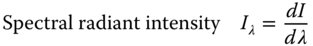
By way of illustration, we will examine the spectral intensity produced by a commonly used illumination source. The xenon arc lamp is extensively used in commercial and laboratory applications as a ‘point source’, with a spectrum similar to that of the sun. Such (nominally) point sources are generally described by their radiant intensity, which gives a useful measure of the overall output of the source. In the case of the spectral measure, spectral radiant intensity is measured in Watts per steradian per nm. Figure 7.4 shows a plot of spectral radiant intensity versus wavelength for a 1000 W xenon lamp.
Similarly, the solar flux arriving at the earth's surface may be denominated in terms of the spectral irradiance – that is the solar flux per unit area of the earth's surface per unit bandwidth. In the case of Figure 7.5, the data presented represents the spectral irradiance of the sun above the earth's atmosphere, as signified by the parameter ‘AM0’ or air mass zero.
Of course, Figure 7.5 does not present the solar irradiance as it would be at the sun's surface; this would be very much greater and would fall off according to the inverse square law, Eq. (7.3). When calculating the spectral radiance associated with the data in Eq. (7.5), one would have to divide the irradiance by the solid angle subtended by the 0.5° solar disc, i.e. 6.8 × 10⁻⁵ sr. Peak solar spectral radiance (at ∼500 nm) would be about 30 000 W m−2 sr−1 nm−1.
7.2.5 Blackbody Radiation
Thermal radiation is associated with the thermal emission of electromagnetic radiation from an incandescent source. In particular, blackbody emission occurs when a solid surface is in thermal equilibrium with the surrounding electromagnetic radiation. The exitance associated with a black body emitter at an absolute temperature of T, is proportional to the fourth power of the temperature and given by the well known Stefan's law:

σ is Stefan's constant (5.67 × 10⁻⁸ W m−2 K−4); ε is the surface emissivity (1 for a perfect black body).
Figure 7.4 Xenon arc lamp spectral intensity.
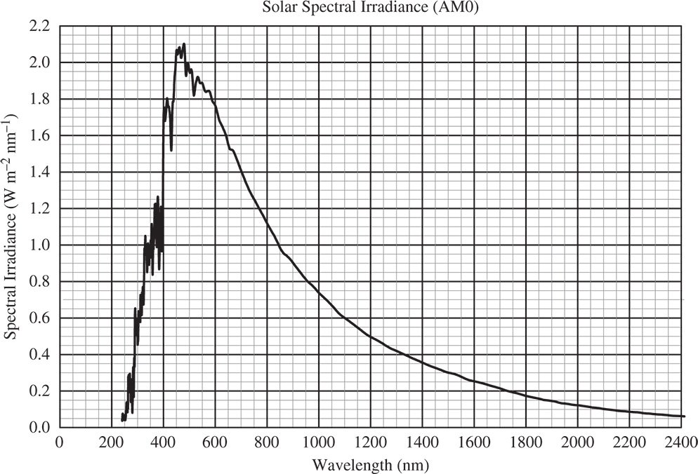
Figure 7.5 Solar spectral irradiance.
Source: NASA SORCE Satellite Data – Courtesy University of Colorado.
Most importantly, blackbody emission has a characteristic spectral distribution, quantified by its spectral radiance which depends only upon the wavelength and the surface temperature. The spectral radiance of blackbody emission is defined by Planck's law:
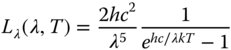
Lλ is expressed in SI units – W m−3 sr−1; h is Planck's constant; c the speed of light; k the Boltzmann constant.
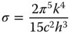
To convert Eq. (7.9) to spectral exitance from a surface, one assumes Lambertian emission and the spectral radiance is multiplied by a factor of π to give the exitance, as per Eq. (7.6). Indeed, the overall radiance and exitance can be obtained by integrating Eq. (7.9) with respect to wavelength. This implies that Stefan's constant is not actually a fundamental unit and can be expressed in terms of more fundamental units, as follows:
Taking the data from Figure 7.5, and using the angular size of the sun, we can plot the data as spectral radiance rather than spectral irradiance. This is illustrated in Figure 7.6. It is quite apparent that the spectral distribution of solar radiance conforms quite closely to that of blackbody emission. For reference, Figure 7.6 shows a plot of 5800 K blackbody emission generated using Eq. (7.9). Thus, to a reasonable approximation, solar radiation can be described as blackbody emission with a characteristic temperature of 5800 K. As stated previously, radiance describes the effective brightness of a surface and, for blackbody emission is purely related to the physical characteristics of the source, temperature, and so on and not to geometry. So, as stated earlier, although the spectral irradiance of solar emission is reduced as one moves away from the sun, the corresponding reduction in the angular size of the sun maintains the spectral radiance at a constant level.
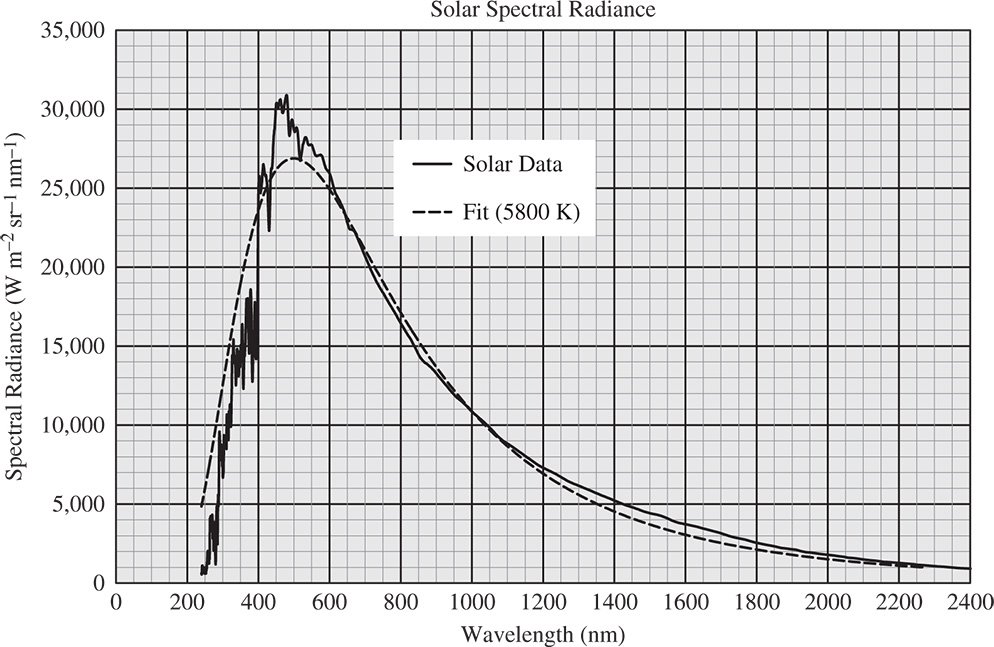
Figure 7.6 Solar spectral radiance and 5800 K blackbody radiance.
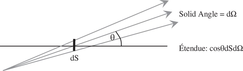
Figure 7.7 Étendue of a pencil of rays.
7.2.6 Étendue
Étendue is the product of the area and solid angle of a pencil of rays in an optical system. The concept of étendue is central to the understanding of the radiometry of an optical system together with many other aspects of optical system performance. As applied to an optical system, its étendue may be represented as the product of the entrance pupil area and the solid angle of the input field. A critical aspect of the behaviour of étendue in an optical system is the operation of the Lagrange invariant. Effectively, the Lagrange invariant and the inverse relationship between linear angular magnification implies that étendue must be preserved in an ideal optical system. That is to say, for a perfect paraxial system, as the imaged (exit) pupil size is increased, the corresponding field angle will be reduced proportionately. Of course, this only applies to a perfect optical system and any image degradation due to aberration has a tendency to increase the étendue. The concept of étendue is illustrated in Figure 7.7.
More formally, as illustrated in Figure 7.7, the étendue of a pencil of rays is given by:
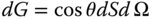
G is the étendue and θ is the tilt of the surface normal with respect to the ray pencil.
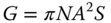
As outlined earlier, for a generalised and perfect optical system, its étendue is a system invariant. Describing the pupil size of a generalised optical system by its numerical aperture, NA and the field by its total area, S, then the system étendue is given by:
The similarity of Eqs. (7.11) and (7.4) which denominates the connection between radiance and flux, brings us to the fundamental utility of étendue in radiometric calculations. It is easy to appreciate that, for an optical system, the radiance associated with a pencil of rays is the derivative of the flux with respect to the étendue.

If the étendue of a pencil of rays is invariant through an ideal system, then the implication of Eq. (7.13) is that the radiance associated with the object and image must be identical. This is very important, as it conveys a fundamental thermodynamic truth. If one considers a blackbody object, any reduction in étendue through the system would imply that the radiance of the image is higher than that of the object. In the context of blackbody radiation, the associated temperature of the image would be higher than that of the object. Therefore, the effect of this would be to take energy from the lower temperature source (the object) and convey it to a higher temperature body (the image) without doing work. This is in violation of the second law of thermodynamics. Any imperfections in the optical system (aberrations) tend to increase the étendue and so reduce the radiance at the image.
The practical utility of étendue lies in its assistance in expediting radiometric calculations in complex optical systems. If one has a source with some known spectral radiance, Lsource, a system with étendue, Gsystem, and a system throughput of ξ, then the flux, Φimage, arriving at the image is simply given by:
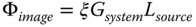
The throughput, ξ, is simply a measure of how much light is transmitted through an optical system as mediated by any scattering, absorption, or reflection that occurs. If, as in the case of an ideal system, none of the optical surfaces were to absorb, scatter or reflect any light, then the throughput would be 100%.
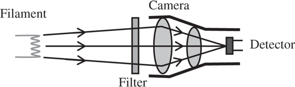
Worked Example 7.1 Flux Calculation
To illustrate the power of the foregoing analysis, we will now examine a practical example. An optical system is designed to view the filament of a tungsten halogen lamp. A camera with an aperture of f#2 images the filament onto the square pixels of a detector; the size of the pixels is 10 μm. For a single pixel of interest, only a small part of the incandescent filament is imaged which fills the entire pixel. The filament itself may be regarded as a blackbody emitter with a temperature of 3000 K. A narrowband filter is included in the optical train which only admits light in a 5 nm wide band around 500 nm. With the exception of the filter, the system throughput, ξ, is 80%. What is the flux arriving at a single pixel?
We are told that the source is a 3000 K blackbody emitter; therefore we should be able to calculate the spectral radiance from Eq. (7.9). In fact, we are interested in the spectral radiance at 500 nm. From Eq. (7.9), the spectral radiance is 2.6 × 10¹¹ W m−3 sr−1 or 260 W m−2 sr−1 nm−1 at 500 nm. The radiance transmitted by the 5 nm bandwidth filter is 5 × 260 or 1300 W m−2 sr−1 at. We now need to calculate the system étendue from Eq. (7.9). The numerical aperture of the system in image space is 0.25 (for f#2) and the area, S, of a single pixel is 10−5 × 10−5 = 10−10 m2.

The solution is now almost complete, we only need to apply Eq. (7.14), making an allowance for the throughput, ξ, of 80%:

Thus, the power arriving at a single pixel is 2.04 × 10⁻⁸ W.
The essential point of the previous analysis is that the same fundamental logic and analysis applies, irrespective of the complexity of the optical system under investigation. In this example, we are not given any details of the optical design, only the pupil and field size. Nevertheless, we are able to estimate the flux arriving at the detector pixel. Of course, we are assuming that system aberrations do not play a significant role.
7.3 Scattering of Light from Rough Surfaces
Much of the preceding analysis has focused on self-luminous sources. These sources, such as blackbody emitters, more or less emit light in a random fashion. In the study of radiometry, we are also interested in surfaces that scatter light in a more or less random fashion. This is distinct from specular surfaces, i.e. mirrors, which reflect light in a deterministic, ordered fashion. The topic was touched on very briefly when we touched on perfect or Lambertian scattering where the radiance of the scattered light is independent of the scattered angle. Unfortunately, this condition is not realised in real materials, so an alternative approach is needed. Here we shall now describe a more generalised treatment, which describes the scattering from a surface using the so-called bi-directional reflection distribution function (BRDF).
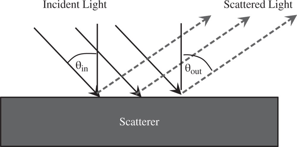
Figure 7.8 Illustration of BRDF.
Light that is incident upon a surface is described by its irradiance and its incident angle, θin, as depicted in Figure 7.8. The scattered light is described by its radiance and its output polar angle, θout. Significantly, since the incident light breaks the symmetry of the scattering surface about the normal, the azimuthal angle, φ, of the scattered light also needs to be described. The BRDF is simply the derivative of the output radiance with respect to the input irradiance.
Naturally, the BRDF is a function of wavelength, so the input irradiance might be defined as E(θin, λ) and the output radiance as E(θout, φ, λ). In this case, the BRDF is given by:
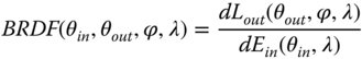
Units for BRDF are sr−1 and a perfect Lambertian scatterer, with a total hemispherical reflectance of unity, would have a uniform BRDF of 1/π. Interest in the radiometry of scattering arises from two principal practical considerations. Firstly, in many applications in optical imaging, there is a requirement to provide uniform illumination over a specific input field. Secondly, there is a diverging motivation in that the optical designer is keen to avoid the deleterious impact of scattered light on image contrast. Therefore, it is important to understand not only the impact of the optical components themselves in manipulating light, but also the effect of the optical mounts and surrounding enclosures and other non-optical surfaces in scattering light.
The preceding chapters have given a clear understanding as to the underlying principles of optical design in so far as the optical components and surfaces are concerned. Ultimately, as will be discussed in detail later, in contemporary design, this proceeds by the use of optical modelling software. For the optical components themselves, the process is referred to as sequential modelling where rays progress in a deterministic fashion and in a clear sequence from one optical surface to the next. In contrast, scattering is an inherently stochastic process, with the scattered distribution described by the BRDF which is essentially a probability distribution for scattering. In the light of these random processes, there is no inherent, ordered sequence of surfaces through which the light progresses. As such, any modelling in this scenario must account for the non-sequential nature of light propagation. Such modelling, of course, must account for the geometrical distribution of any scattering and the study of BRDF distributions is of considerable practical utility.
An example of the BRDF of a real material, Spectralon®, is shown in Figure 7.9. The data is for a wavelength of 900 nm and normal incidence, i.e. θin = 0. Spectralon, is based upon sintered polytetrafluoroethylene (PTFE) and represents the closest approximation to an ideal scatterer of any material. Even so, there is a tendency for the BRDF to decline with increasing polar angle.
7.4 Scattering of Light from Smooth Surfaces
The foregoing analysis is entirely appropriate for the scattering of light from matt or rough surfaces. However, polished surfaces, such as those in lenses and mirrors, can contribute to the unintended scattering of light, even though their roughness is very low. Analysis of this type of scattering is of exceptional importance where low levels of stray light might degrade faint images. For such surfaces, it is useful to quantify the roughness of the surface in terms of the root mean square roughness, σrms, which expresses the rms departure of the surface from the ideal surface, whether that be a plane, spherical, or aspherical surface. This is illustrated in Figure 7.10, showing the high spatial frequency departure from the nominal shape.
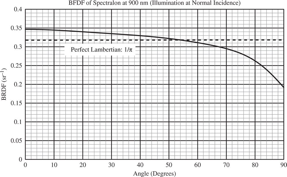
Figure 7.9 BRDF of Spectralon at 900 nm for normal illumination.
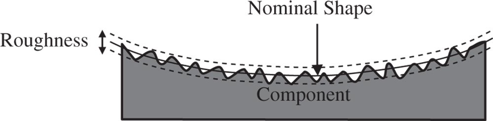
Figure 7.10 Surface roughness.
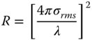
For polished optical surfaces, such as mirrors and lenses, σrms is very low, typically a fraction of a nanometre. The surface roughness is thus a very small fraction of the wavelength of light and, in this case, surface scattering may be presented as a diffraction problem. That is to say, a perfect surface would produce the reflection of a perfect wavefront and the surface roughness imposes a wavefront error equal to twice the surface roughness (due to the reflective double pass). In classical diffraction analysis, we would analyse the additional wavefront error induced in terms of the image quality degradation. That is to say the scattered light caused by the departure from nominal surface shape would cause some kind of change in the clarity of the image itself. However, in the case of surface roughness, the scattered light is considered entirely separately from image degradation. In terms of the departure of the surface from the nominal shape, only high spatial frequency variations are considered to contribute to scattering and are included in the definition of surface roughness. If Fraunhofer diffraction is considered, then the high spatial frequency components of surface roughness scatter the light far away from the nominal image. As such, this produces an irradiance distribution that is clearly separated from the imaged spot at the image focal plane. In practice, spatial wavelengths of less than 0.1–1.0 mm are considered as surface roughness; longer wavelength departures are analysed as ‘form error’ and contribute to image degradation. The analysis of scattering proceeds in a similar way to the calculation of the Strehl ratio (Chapter 6) for small system wavefront errors and gives a total hemispherical reflection of:
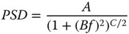
It is tempting to proceed with an analysis of scattering on the assumption that this ‘small signal’ scattering is Lambertian in character. However, this is very far from the truth. The angle of scattering, from simple Fraunhofer diffraction analysis is proportional to the spatial frequency of the surface roughness component. Of course, Fourier analysis may be used to express the roughness deviation of any surface in terms of the sum or integral of a series of sinusoidal terms of varying frequency. The random surface roughness of the type depicted in Figure 7.10 may be thus analysed and its power spectrum (i.e. square of the amplitude) may be expressed as a power spectral density (PSD) as a function of spatial frequency. As such, the PSD represents surface deviation power per unit spatial frequency bandwidth. The ‘power’ of a surface deviation is proportional to the square of the amplitude and might be measured in mm2 and since the surface is represented by Fourier components in two dimensions (x and y), spatial frequency bandwidth might be measured in mm−2. Therefore, for an area based description, as opposed to a linear one, PSD has dimensions of length4, e.g. mm4. The relevance of this discussion is for all polished surfaces, the PSD falls off very rapidly with spatial frequency and, as a consequence, the scattering amplitude or BRDF diminishes rapidly with angle (with respect to the main beam).
To a reasonable approximation, the PSD follows an inverse power law dependence upon spatial frequency. For a two dimensional Fourier description, for typical polished surfaces, this power law exponent is around −3. In the corresponding linear Fourier description, which is sometimes used, this exponent is around −2 and the PSD dimensions are mm3, rather than mm4. However, in this text we will retain the two dimensional description. Figure 7.11 shows an idealised PSD spectrum for a polished surface with nominal frequency exponent of −3. The total integrated surface roughness for the plot in Figure 7.11 is 5 nm rms. Apart from the simple exponent in Figure 7.11, we have introduced a ‘corner frequency’, f0, where the PSD reaches a maximum value. Without the introduction of a corner frequency, the integrated roughness would tend to infinity when the integral proceeds to zero spatial frequency. In the context of our discussion on scattering, this corner frequency relates more to the somewhat arbitrary demarcation between scattering and image degradation, as previously outlined. This boundary may typically be between spatial frequencies of 1 and 10 mm−1 or spatial wavelengths between 0.1 and 1 mm.
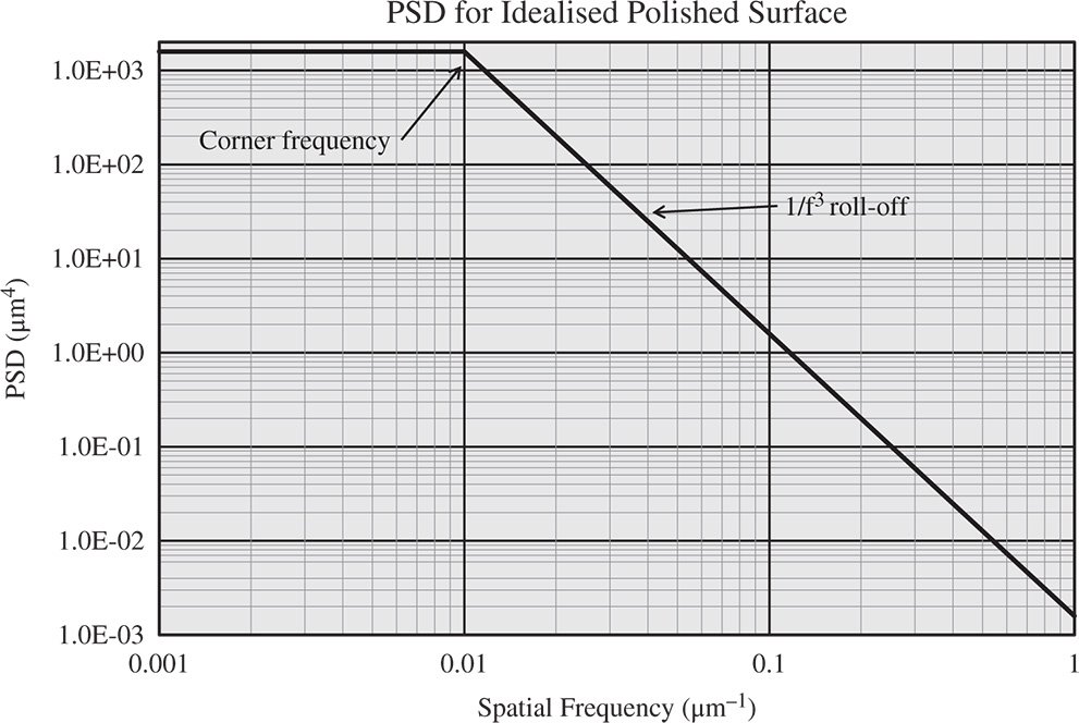
Figure 7.11 PSD for idealised polished surface (note units are in microns).
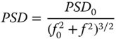
With the introduction of the corner frequency, f0, surface roughness power dependence upon spatial frequency may be modelled in a very specific way, as set out in Eq. (7.17):
A more generalised formulation of Eq. (7.17) is the so-called k correlation model which introduces the ABC parameters:
In our specific model, as outlined in Eq. (7.17), the C parameter in Eq. (7.18) is three. The parameter, B, is effectively the inverse of the corner frequency. In terms of the utility of this model with regard to scattering, the spatial frequencies may be directly translated into scattering angles or, more strictly, the sine of the scattering angles. As a consequence, the ABC model may be re-cast to given an explicit solution for the BRDF in terms of the scattering angle, θ:

Of course, the ABC coefficients in Eq. (7.19) are not the same as those in Eq. (7.18). Equation (7.19) may be integrated across all polar angles to give the total hemispherical reflection. This gives:
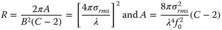
Equations (7.19) and (7.20) gives us the ability to model scattering from mirror surfaces. However, when modelling the direct scattering from lens surfaces, we must replace Eq. (7.16) for the hemispherical scattering with the following equation:
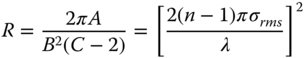
In Eq. (7.21) for a lens surface, the optical path difference is represented by the product of (n − 1) and the form error, as opposed to twice the form error, as in a mirror. As such, Eq. (7.21) gives a clear indication that the scattering from lens surfaces is much less than that from mirrors. For example, for a lens material with a refractive index of 1.5, the total scattering is diminished by a factor of 16 when compared to a mirror.
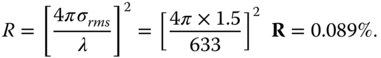
Worked Example 7.2 A polished mirror has a surface roughness of 1.5 nm rms. We are interested in its scattering at a wavelength of 633 nm. For the purposes of subsequent analysis, we may assume that the C exponent has a value of 3. In addition, the corner frequency may be assumed to be 4 mm−1. What is the total hemispheric reflection at the designated wavelength? Calculate the A and B coefficients.
The total hemispheric reflection is given by Eq. (7.16). We are told that σrms = 1.5 nm and λ = 633 nm.
The corner frequency, f0 is 4 mm−1 and the B coefficient is given by the simple Eq. (7.19):
Finally, from (7.20) we have: