


Полная версия
Optical Engineering Science
Worked Example 6.3 – Beam Divergence of a Fibre Laser
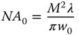
A laser beam with a wavelength of 1.55 μm emerges from a single mode fibre. The laser beam, at this point can be characterised as a beam with a waist size of 5.25 μm. What is the characteristic numerical aperture, NA0, associated with the far field divergence?
Substituting the relevant values into Eq. (6.28), we get:
The numerical aperture is thus 0.094 and this corresponds to a divergence angle of 5.39°.
Expressed as a FWHM, the near field beam width is 6.18 μm, and the rms radius is 4.37 μm. Similarly in the far field the FWHM divergence angle is 6.35° and the rms divergence angle is 3.81°.
6.7.2 Gaussian Beam Propagation
Thus far, we have analysed the relationship between the near field and far field dispositions of a Gaussian beam. We now turn to the more general case of the propagation of a Gaussian beam. As in the previous analysis, the laser beam is defined by a characteristic Gaussian radius. In this case, the characteristic radius, w(z), is a function of the axial propagation distance, z. To describe the laser beam, we introduce an envelope function, A0(x, y, z) that describes the radial profile of a propagating laser beam.
In practice, in most cases, the size, w(z), of the laser beam is much larger than the wavelength, and we can use the slowly varying envelope approximation. This is, in effect, a paraxial approximation, where far field divergence angles are necessarily small and can be formally expressed as:
(6.30)
Applying Eq. (6.29) to the scalar version of Maxwell's equation and taking into account the above approximation, we obtain the so-called paraxial Helmholtz equation:

As suggested, in the case of a Gaussian beam, the amplitude may be expressed a characteristic width, w(z) which varies slowly with respect to z. Most significantly, w(z) can be complex, giving rise to wavefront curvature. This may be easily seen if the complex part of the envelope is subsumed within the sinusoidal propagation term, leading to a quadratic phase variation across the beam. In the Fresnel and paraxial approximation, these quadratic wavefronts may be viewed as approximately spherical. This is illustrated in Figure 6.12.
Mathematically, the Gaussian beam envelope is expressed as follows:
The component A0(z) represents the peak on axis amplitude and this would be expected to diminish as the beam expands. To make the analysis more tractable, we subsume this axial variation into the exponential function as a complex function of z, β(z). Furthermore, both real and imaginary parts of the Gaussian are combined into a single complex function, α(z). Hence, to solve the paraxial Helmholtz equation in this instance we re-cast Eq. (6.32) in the following form:
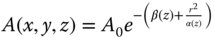
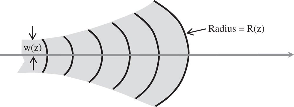
Figure 6.12 Gaussian beam.
And substituting this into the paraxial Helmholtz equation:
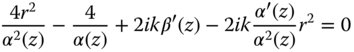
This equation must hold for all values of r. Both the quadratic terms and those with no dependence in r must sum to zero. Taking the quadratic element only, we may derive a very simple relationship for α(z).

By viewing Eq. (6.32) it is straightforward to relate β(z) to the beam size, w(z) and the radius R(z):
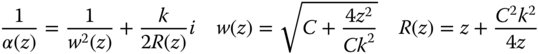
To interpret the constant C, we assume that there exists a minimum beam size, the beam waist, where the wavefront curvature is zero. We denote this beam waist by the symbol, w0. It is clear, then, that the constant C is equal to the square of the beam waist. Eliminating the constant, C, gives:
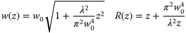
We note that there some characteristic distance, Rz, over which the beam expands around the beam waist. This distance is known as the Rayleigh distance and the Eq. (6.35) may be finally re-cast to give the following:
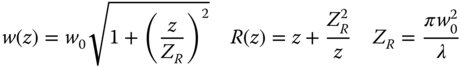
The Rayleigh distance is of particular significance. In effect, it sets the demarcation between the near field and the far field. In the case of the far field, z ≫ ZR the expressions in Eq. (6.36) revert to the Fraunhofer diffraction pattern of a Gaussian beam:
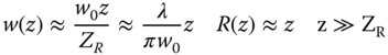
This may be compared with Eq. (6.28) and is very similar in form. Thus Eq. (6.37) represents the far field diffraction pattern of a Gaussian beam. In the near field where z ≪ ZR, the beam is parallel and the size constant at w0 and, of course, the radius tends to infinity. At the Rayleigh distance, the beam size is increased by a factor corresponding to the square root of two and the wavefront radius is equal to twice the Rayleigh distance. This is illustrated more formally in Figure 6.13.
For values of z that are of a similar magnitude to the Rayleigh distance, then the beam is in an intermediate zone between the near and far fields.
Worked Example 6.4 – Rayleigh Distance of Fibre Laser
In the previous worked example, we introduced a fibre laser with a wavelength of 1.55 μm, with a Gaussian beam size of 5.25 μm. If we assume that the beam waist is located at the exit from the fibre, what is the Rayleigh distance of the laser beam? In addition, what is the beam size, w(z), 50 μm from the exit from the fibre and what is the wavefront radius at that location?
From Eq. (6.36):
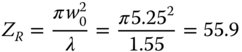
The Rayleigh distance is 55.9 μm
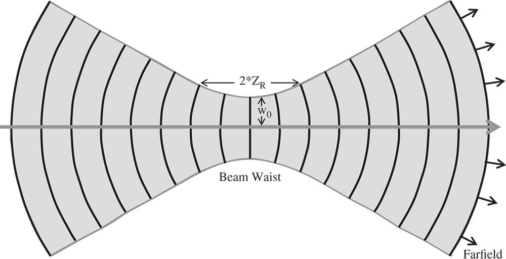
Figure 6.13 Form of expanding Gaussian beam and beam waist.
Calculation of the beam size and the wavefront radius also proceeds from Eq. (6.36).
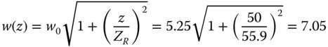
The beam size, w(z), is 7.05 μm
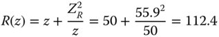
The wavefront radius is 112.4 μm
6.7.3 Manipulation of a Gaussian Beam
The preceding analysis has presented an analysis of the propagation of a Gaussian beam through free space. However, in most practical instances, the beam will be manipulated by optical components, lenses, and mirrors and so on. Therefore it would be useful to be able to understand the impact of an individual optical component or system on the propagation of a Gaussian beam. In the analysis presented here, the component or system is simply represented in its paraxial form by a ray tracing matrix, as presented in Chapter 1. The matrix is populated by four elements, A, B, C, and D and these transform the wavefront radius according to the following equation:
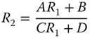
(R1 and R2 are the input and output radii respectively)
For a Gaussian beam, the wavefront curvature can be represented by the complex quantity, q, where q = z + iZR. The distance from the beam waist is represented by z and ZR is the Rayleigh distance. Expression (6.38) may be re-cast in the following form:
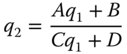
where q = z + iZR
This is the so-called ABCD law for the manipulation of Gaussian beams.
Worked Example 6.5 – Gaussian Beam Manipulation
A helium neon laser beam at 633 nm has a beam waist of 0.6 mm, located 80 mm from a positive lens of focal length 60 mm. Calculate the size of the beam waist following the lens and its location with respect to the lens.
If we take the origin of the co-ordinate system to be at the original beam waist (z = 0), then the system matrix consists of a translation by 80 mm followed by a 60 mm focal length lens.
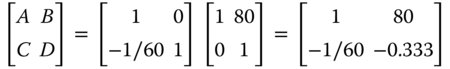
A = 1; B = 80; C = −0.0167; D = −0.333
The Rayleigh distance of the original beam is given by:
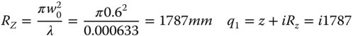
Using the ABCD law:
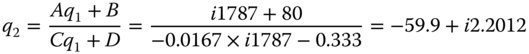
The lens lies at −59.9 mm from the beam waist and hence the beam waist is 59.9 mm in advance of the lens. The Rayleigh distance is 2.201 mm. This corresponds to a beam waist size (from Eq. (6.36)) of 0.02 mm or 20 μm.
The new beam waist lies approximately at the focus of the lens. Since the lens lies much closer to the original beam waist than the corresponding Rayleigh distance, then the beam is almost parallel and the new beam waist should lie very close to the focal position.
6.7.4 Diffraction and Beam Quality
All the analysis presented thus far has assumed a Gaussian beam that possesses perfect spatial coherence. Perfect spatial coherence implies that an unambiguous phase relationship exists between all points across the wavefront. A less than perfect wave disturbance is composed of a number of different components whose phase relationship is entirely random. As such, spatial coherence is defined more formally as the correlation between the wave disturbance at two points. The complex amplitude of a wave at a point, A(t), may be expressed in Fourier space in terms of a frequency distribution, S(f). The coherence between two points, x, y is simply given by the cross correlation of the two disturbances:
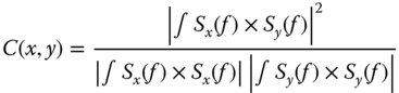
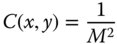
Perfect coherence is represented by a correlation of one; complete incoherence is represented by a correlation of zero. In many practical problems in Gaussian beam propagation, it may be assumed that the coherence of the laser beam is one. However, this is dependent upon the number of independent ‘modes’ that characterise the laser beam. A single mode is effectively one unique solution to the wave equation and laser devices are often engineered in such a way that only one of these modes is allowed to propagate. The extent to which this is true is a measure of the laser's beam quality. The beam quality of a laser is generally expressed by the parameter M2or M squared and is indicative of the number of modes supported by the beam. If this value is one or close to one, then the beam quality is high and any propagation analysis will proceed as previously described. For a beam with a beam quality defined by the M2 parameter, then the spatial coherence is given by:
Returning to the practical question of Gaussian beam propagation, the beam propagation may be expressed entirely in the original form given by Eq. (6.36), except with a revised Rayleigh distance, Z′R.
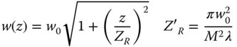
It is clear from Eq. (6.42), that, where M2 is significantly greater than one, the divergence of the laser beam in the far field is greater than would be expected from a perfect beam. The revised equivalent of 5.68, giving the beam divergence is set out in Eq. (6.43).
In practice, the M2 value for a laser beam is measured and then analysed using the relationships set out in Eqs. (6.42) and (6.43). The parameter is generally specified for many commercial laser systems.
6.7.5 Hermite Gaussian Beams
Further exploring the theme of multiple modes as individual solutions to the wave equation, we must recognise that the simple Gaussian beam previously defined is not the only solution to the paraxial Helmholtz equation. In fact, a complete set of orthonormal solutions exist of which the simple Gaussian solution is the first member. Orthonormal, in this context, means that the cross-integral of two different solutions is always zero and that involving the same solutions is always unity. This is an important property, as will be seen later. This set of solutions are defined by the Hermite-Gaussian polynomials, where the original Gaussian amplitude envelope is multiplied by a unique Hermite polynomial in x and y. Each Hermite polynomial solution is defined by its maximum order in x and y, which we will refer to as l and m respectively. Overall, the solution may be represented as:

The expression w(z) is simply the Gaussian beam radius for any specific value of z, as given in Eq. (6.36) and A[w(z)] is a normalising factor. The first few polynomials are set out Table 6.1.
Figure 6.14 shows graphically the form of some low order Hermite polynomials.
The orthogonal nature of the polynomials provides a suggestion as to their utility. As with a Fourier series, any arbitrary beam profile may be represented as a summation of a series of Hermite polynomials. If we represent the full expression contained in Eq. (6.44) as Gl,m(x, y, z), then the series may be represented as:
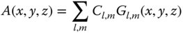
Cl,m are coefficients describing the amplitude of each term
Table 6.1 Low order Hermite polynomials.
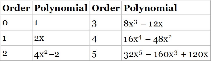

Figure 6.14 A selection of low order Hermite polynomials.
Assuming the beam profile is known as some plane, z0, then each coefficient may be calculated by exploiting the orthonormal property of the series:
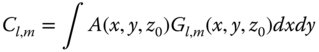
Thus, Gaussian-Hermite polynomials represent a powerful tool for physical optics propagation. Assuming a beam profile is known at some point, the relevant coefficients may be calculated according to Eq. (6.46) and summed according to Eq. (6.45) and then propagated in free space according to Eq. (6.44).
6.7.6 Bessel Beams
An interesting solution to the paraxial Helmholtz equation, Eq. (6.31), is the so-called Bessel beam. Generally, Bessel functions of the first kind form a series of solutions to the equation. Most specifically for an axially symmetric form, the solution is represented by a Bessel function of the first kind and zeroth order. The unique feature of this solution is that the wavefronts are planar and the amplitude envelope of the beam does not change as it propagates. That is to say, the beam appears to be diffractionless and does not diverge. The solution is of the form given by:
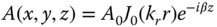
J0 is a Bessel function of the first kind and zeroth order;
Another interesting type of beam is the Talbot beam. Rather than retaining a constant profile as it propagates, the Talbot beam replicates itself at specific propagation distances. For further details, the reader is advised to consult the Further Reading section at the end of the chapter.
6.8 Fresnel Diffraction
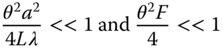
The study of Gaussian beam propagation has provided us with a more quantitative description of near field and far field propagation and where the boundary between the two zones occurs. In our analysis of Fraunhofer diffraction, we considered only the far field approximation. Related to the concept of the Rayleigh distance for Gaussian beam propagation is a dimensionless parameter called the Fresnel number. If the near field is defined by some aperture with a radial dimension of a, then the Fresnel number, F, at a propagation distance of L from the aperture is given by:
Referring to Eq. (6.36), then the Gaussian beam equivalent of the Fresnel number is the ratio of the Rayleigh distance, ZR, to the beam propagation distance. For Fresnel numbers much less than one, then the diffraction pattern may be considered as a far field pattern and the Fraunhofer approximation applies. Where the Fresnel number is much greater than one, then one is in the near field.
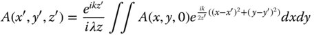
The analysis of Fresnel diffraction is derived from the Rayleigh diffraction formulae (Eqs. [6.8] and [6.9]). The key assumption in the Fresnel analysis relates to an approximation of the propagation distance, s. If one assumes that the near field object is located at z = 0, then the propagation distance may be approximated in the following manner:

In making the above approximation, based on a Taylor series expansion, we are choosing to ignore terms of fourth order in x and y. These terms cannot be permitted to make a significant contribution to the phase when the approximation is applied to the Rayleigh formulae. Setting out the fourth order terms more explicitly, it is straightforward to delineate the approximation more clearly:
If we re-cast z as the propagation distance, L, and represent the ratio x/z as θ, the angular size of the near field and also denominate the near field radius as a, then the Fresnel condition is given by:
The value of the Fresnel approximation is that it now permits us to treat the axial propagation distance, z, as a constant and to remove it from the integral in the diffraction equation, producing a more simple expression involving integration with respect to x and y. This is the so-called Fresnel integral and it is set out below.
It would be useful, at this point, to illustrate the assumptions underlying Fresnel diffraction with a practical example. An optical system populated with components with a standard diameter of 25 mm would have an effective radius of 12.5 mm. For a wavelength of 500 nm, the Fresnel approximation applies to distances much greater than 250 mm. At that distance, the Fresnel number is about 1000, so we are clearly in the near field zone.
To illustrate the application of Fresnel diffraction, we might now apply it to a uniformly illuminated slit of width w. Without loss of generality, this provides a simple illustration of the application of Fresnel diffraction in one dimension. For a given source point, e.g. x = 0, then the phase of the sinusoidal component of Eq. (6.51) is of critical interest. In particular, we are concerned with points where the phase expressed in Eq. (6.51) is a half period number of waves. That is to say:
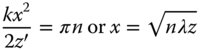
The effect of diffraction at an edge or an aperture is to produce an alternating series of light and dark rings. The disposition of these rings is affected by the relative phases of contributions from the source. As such, Eq. (6.52) provides some indication of the location of these rings. The locations of these points, as set out in Eq. (6.52) are referred to as the Fresnel zones. Based on application of Eq. (6.51), for the one dimension, the diffracted amplitude from the slit is proportional to:
We make the substitution s = x − x′ and make the further assumption that the diffraction pattern is symmetrical about the centre of the slit. In doing this, we may be permitted, without loss of generality in assuming that x > 0. The integral now becomes:
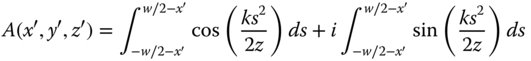
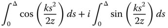
We will now refer to the quantity w/2 − x′ as Δ. The quantity Δ now represents the distance in x from the positive edge of the slit.

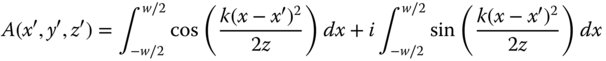
The sign of the first and third terms in Eq. (6.55) is dependent upon the sign of Δ. If Δ is greater than 0, then the sign is negative and vice versa. The structure of the integral above is of great importance, as it can be decomposed into two relatively simple integrals of the form:
The above integral is of great importance and is known as the Fresnel integral. Plotting both components of amplitude in Figure 6.15, we produce the familiar form of the Cornu spiral.
Progression around the Cornu spiral in Figure 6.15 is marked by increasing values of Δ, the distance from the slit boundaries. Each successive Fresnel zone is marked in Figure 6.15 and the numbering of the zones is as per Eq. (5.52). Most importantly, it is clear from Figure 6.15 that an asymptote is reached for large values of Δ. At large values of Δ, the integral tends to 0.25 + 0.25i. If, in Eq. (6.55), one assumes that w-Δ is large, then this asymptotic value must be added to the integral. In this case, we can now reasonably approximate the integral expression in Eq. (6.55) in the following manner:
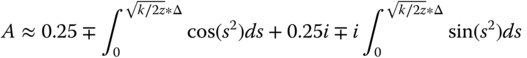
When Δ is large and positive, the integral part of Eq. (6.57) cancels out the constant asymptotic values, so the amplitude is zero. Of course, that the amplitude is zero away from the illuminated portion of the slit is to be expected. In the opposite scenario, where a position within the illuminated area is viewed, then the flux levels tend to a uniform value. Around the edge position, and towards the illuminated area, a series of light and dark bands emerge. One can see from the disposition of the Cornu spiral, that the contrast of these bands diminishes as the effective Fresnel zone number increases and, from Eq. (6.52), they also become more tightly packed.