

Полная версия
Optical Engineering Science
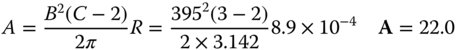
Thus, in the full representation, A = 22.0, B = 395, and C = 3.
In terms of practical application, models such as the ABC model are extremely useful in the validation of designs, such as cameras and telescopes where restriction of scattered light is of paramount importance. This topic will be considered further when we look in more detail at the optical design process in later chapters.
7.5 Radiometry and Object Field Illumination
7.5.1 Köhler Illumination
Hitherto, in all discussions of image formation, no attention has been paid to the illumination of the object. It is assumed, quite arbitrarily, that the object spontaneously emits rays. This may be perfectly proper for a self-luminous object. However, in many cases, the object is not luminous and needs to be illuminated evenly across the entire field. The earliest investigation of this problem is due to August Köhler, resulting in the development of the Köhler illumination system, still in use today. Most light sources, such as filaments lamps or arc sources have a highly spatially non-uniform irradiance. Traditionally, Köhler illumination was developed with a filament lamp source in mind. In this scheme, the light from the filament is collected by two lenses, the collector lens and the condenser lens and presented to the object. However, instead of imaging the filament at the object, which would produce uneven illumination, the filament is imaged at the nominal pupil location which it overfills. The Köhler illumination scheme is shown in Figure 7.12.
The field stop is located close to the collector lens which images the filament onto the aperture stop location. The condenser lens is separated from the aperture stop by its focal length and thus images the filament at the infinite conjugate. In this way, the object plane is uniformly illuminated. Of course, the pupil itself is not uniformly illuminated. However, this is not an impediment to image formation, provided the pupil is well filled. Uniform illumination of both image and pupil conjugates from an uneven source, such as a filament can only be achieved through division of amplitude, e.g. by scattering. This will be dealt with in the next section.
7.5.2 Use of Diffusers
The problem with using an imaging system for illumination, as in Köhler illumination, is that the uneven illumination source must be imaged at some conjugate in the system. This problem may be circumvented by use of a diffusing component within an optical system. Diffusers scatter light in a random but controlled fashion and take the form of transmissive components, such as ground glass screens and opal diffusers, and reflective screens, such as Spectralon diffusers. Reflective materials can approach Lambertian behaviour, but transmissive materials such as ground glass scatter light into relatively narrow angles. Ground glass screens produce a broadly Gaussian BRDF distribution with a full-width half-maximum scattering angle of between 5° and 20° depending upon the coarseness of the ground surface. ‘Engineered diffusers’ based on diffractive surfaces, can be used to create tailor made scattering profiles, such as a top hat profile, where the scattered flux is constant up to a specific scattering angle whence is falls to zero. Figure 7.13 shows the scattering profile of some diffusers.
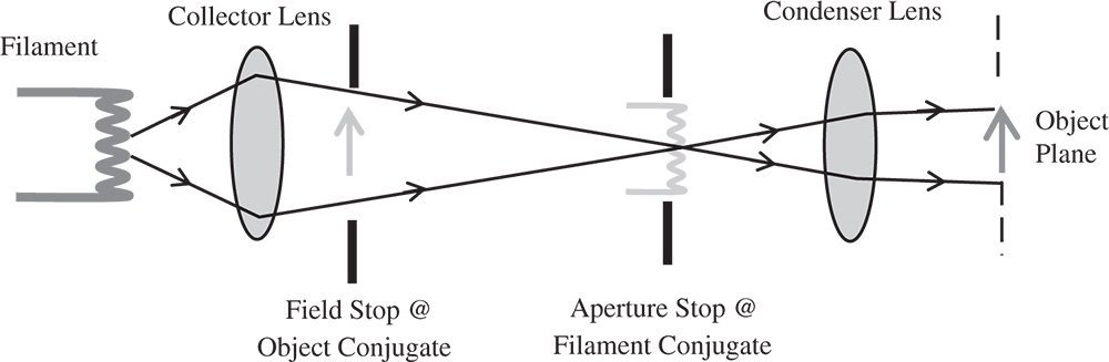
Figure 7.12 Köhler illumination.
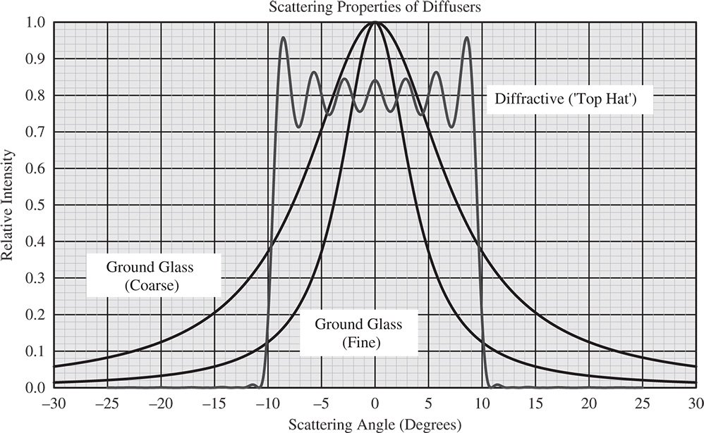
Figure 7.13 Diffuser scattering profile.
Overall, diffusers are very useful in re-arranging light by division of amplitude to promote even illumination. However, it must be understood, in a radiometric context, that diffusers inevitably increase system étendue and their use is inevitably accompanied by a significant reduction in radiance at the final image plane.
7.5.3 The Integrating Sphere
7.5.3.1 Uniform Illumination
Some exacting technical applications require the creation of highly uniform illumination across a field. This is particularly the case in instrument calibration, where even illumination to better than ±1% might be required. Such even illumination may be provided by an integrating sphere. An integrating sphere consists of a spherical cavity coated with some high reflectivity, diffusing material. The sphere is provided with a number of ports, which are apertures in the spherical shell and significantly smaller than the sphere diameter. One of these ports is designated as the input port and one as the output port. The design of the integrating sphere is such that input and output ports are not intervisible and light can only reach the output port by scattering off the internal walls of the integrating sphere. This is shown in Figure 7.14.
The internal coating of the integrating sphere is made of some nominally white coating that scatters efficiently. Traditionally, classic white paint pigments, such as titania (TiO2) and barium sulphate (BaSO4), were used. More recently, this has been replaced by Spectralon (sintered PTFE) for ultraviolet and visible applications and gold coating for infrared applications. These materials have a hemispherical reflectance of over 99% over wide regions of the spectrum. The integrating sphere is designed with a combined port area much smaller than the internal surface area of the sphere. In this way, before exiting the output port, the light must undergo a large number of scattering events. For Lambertian scattering at some point on the internal surface of the sphere, it can be demonstrated, for a spherical geometry, that the irradiance produced at other points of the sphere is entirely uniform.
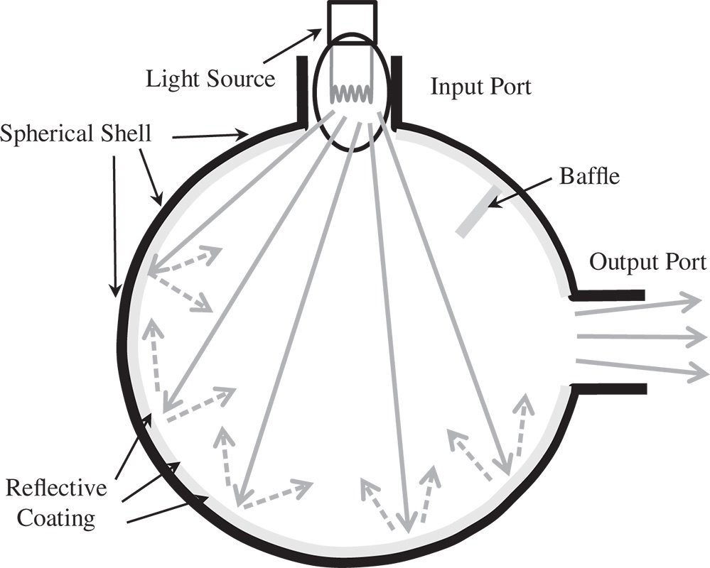
Figure 7.14 Integrating sphere.
However, in practice, no real material is perfectly Lambertian. Nevertheless, in theory, for an infinite number of scattering events, the radiance distribution of the light exiting the output port tends to the Lambertian distribution, even if the internal coating is non-Lambertian. Therefore, as the area of the ports is reduced, as a fraction of the sphere area, then the emission from the output port becomes more Lambertian. As a rule of thumb, the port area should make up no more than 5% of the total sphere area. Thus, for a reasonably small port fraction, the integrating sphere has the property of considerably enhancing the Lambertian quality of the emission from the output port, over and above that of the reflective coating of the sphere itself.
If a light source injects a specific flux into the integrating sphere, as indicated in Figure 7.13, then the irradiance seen at a point on the sphere's surface is not merely the flux divided by the internal area of the sphere. By making the assumption that the integrating sphere is effective in promoting uniform internal illumination, the internal irradiance may be calculated by assuming the flux input is balanced by flux loss from the ports and absorption in the sphere coating. If the internal area of the sphere, including port area, is A, the fractional area occupied by the ports, f, the reflectivity of the sphere coating, R, and the flux input, Φ, then the internal irradiance, E, is given by:

The quantity M is the so-called ‘multiplier’. In practice, for many integrating sphere applications, R > 0.99 and thus M is approximately the inverse of the port fraction. Thus, with a port fraction of 5%, the multiplier is 20. That is to say, the internal irradiance is 20 times greater than would be expected from dividing the flux by the sphere area. The 5% port area restriction means that the port diameter should be smaller than 45% of the sphere diameter and less than a third of the sphere diameter for two ports, and so on.
It is clear that the integrating sphere delivers uniform radiance at the output port. By providing the integrating sphere with a calibrated source, or by calibration of its output radiance and irradiance, it can provide a standard calibrated (spectral) radiance.
7.5.3.2 Integrating Sphere Measurements
By integrating flux uniformly over a large solid angle, integrating spheres can provide an unbiased measurement of flux for diverging sources. That is to say, the integrating sphere integrates emission from these sources across all angles. Examples of such sources might include light emitting diodes (LEDs) and incandescent lamps, and so on. In such measurements, radiation from a lamp is directed into the input port with a photodetector situated at an exit port. This setup is illustrated in Figure 7.15a. In this example, the source is placed at the input port, although for lamps, the source is often placed inside the sphere. A detector placed at the output port is used to monitor integrating sphere radiance. By calibrating the detector using a source (e.g. laser) of known flux, the absolute flux may be calculated. Figure 7.15b illustrates the principle of (total) reflectance measurement. A source irradiates a sample situated opposite the input port. Again, a detector at the output port monitors the integrating sphere radiance. Reference reflectors of known reflectivity are available and such reflectors may be substituted for the sample for calibration purposes. Comparison of the two measurements will give the reflectivity of the sample.
7.5.4 Natural Vignetting
In many respects, the Lambertian illumination of an entrance pupil as would be provided by an integrating sphere represents an ideal situation. However, the irradiance produced at an image plane is actually non-uniform, assuming perfect imaging. In this context, ‘perfect imaging’ means perfect replication of the entrance pupil at the exit pupil. The effect described is known as natural natural vignetting. In the perfect realisation of this phenomenon, the irradiance produced at the image plane is proportional to the fourth power of the cosine of the field angle. The logic of this is illustrated in Figure 7.16.
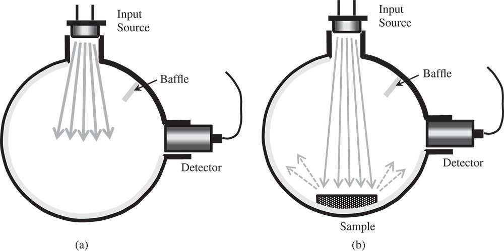
Figure 7.15 (a) Flux measurement. (b) Reflectance measurement.
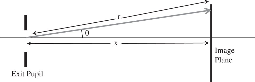
Figure 7.16 Natural vignetting.
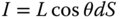
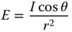
If the (Lambertian) radiance at the exit pupil is L, from Eq. (7.5), the radiant intensity emerging at a normal angle of θ from an area element, dS, of the pupil is given by:
However, from the inverse square law Eq. (7.3) we know that the irradiance produced at the image plane is equal to:
θ is the angle of the ray to the image plane normal (same as angle to pupil normal)
Since r = x/cos θ, we finally arrive at the following relationship for natural vignetting:
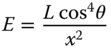
Equation (7.23) summarises the phenomenon of natural vignetting. The reason for the term ‘natural vignetting’ is this effect replicates artificial vignetting, i.e. the darkening of an image towards the edges of a wide field caused by obstruction of light by physical apertures, other than the main stop. In the case of natural vignetting, however, there is no physical obstruction of the light path.
7.6 Radiometric Measurements
7.6.1 Introduction
In any real application, we are interested in the measurement of radiometric quantities, such as irradiance and radiant intensity. However, absolute measurements of these quantities are, in practice, extremely challenging. As an example, absolute measurement of flux or irradiance and so on to ±1% represents a high precision measurement. Although calibration plays an important role in any measurement, this is especially true for radiometric measurements. Absolute radiometric measurement generally proceeds by the use of calibrated detectors. These detectors convert the optical flux into an electrical or thermal signal which can be directly monitored. Critically, the sensitivity of these detectors has been carefully calibrated using a reference source providing a known spectral output. Hence, the signal can be directly converted into flux or radiance, and so on. The reference sources are generally maintained by, or derived from, National Measurements Institutions (NMIs), such as the National Physical Laboratory (NPL) or the National Institute of Standards and Technology (NIST).
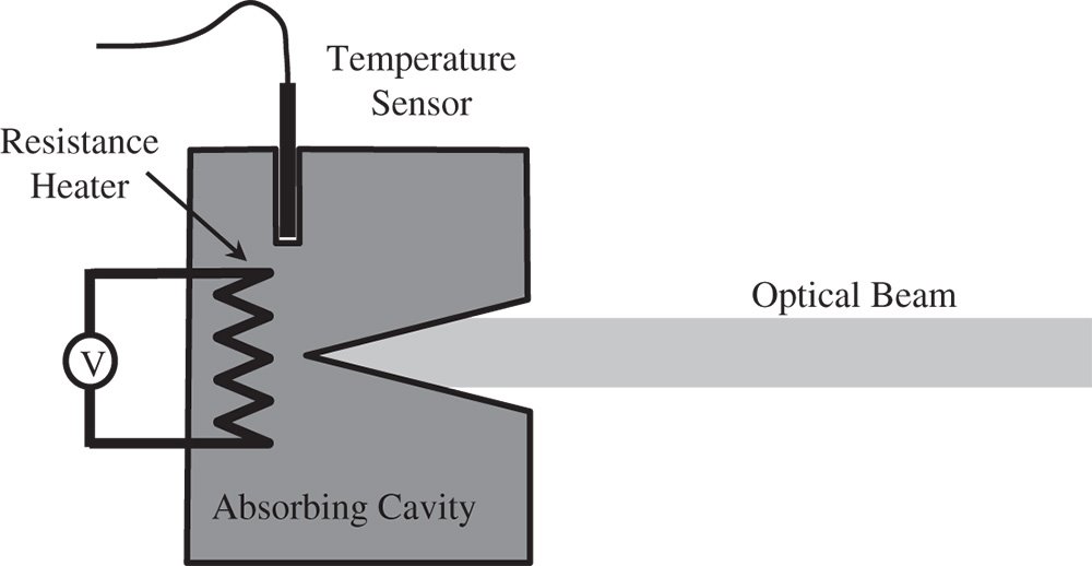
Figure 7.17 Substitution radiometer.
7.6.2 Radiometric Calibration
7.6.2.1 Substitution Radiometry
Calibrated measurements of optical flux are ultimately derived from the principle of substitution radiometry. In this measurement, optical radiation is wholly absorbed in a specially designed black cavity and the temperature increase measured by a thermal transducer. Thereafter, the optical power is substituted by electrical input derived from a resistance heater. The original optical flux is given by the electrical input required to produce the same temperature change. The principle is illustrated in Figure 7.17.
The optical beam in Figure 7.16 may, for example, be derived from a stabilised laser beam. This laser beam, thus characterised, may then be used to calibrate the sensitivity of a detector. Ultimately, the temperature rise with respect to the surroundings provides the signal for this measurement. As a consequence, any drift in the ambient temperature interferes with the fidelity of the measurements. For this reason, the highest precision measurements are obtained with a cryogenic radiometer, where the cavity, sensor, and heater are enclosed within a vacuum and cooled to a few degrees Kelvin.
7.6.2.2 Reference Sources
The primary reference source for flux, or rather for spectral irradiance, is a carefully maintained blackbody source. For the ultraviolet, visible, and near infrared spectral regions, the blackbody source is based upon a pyrolytic graphite cavity. Such sources can operate up to a temperature of 3500 K. In order to capture the spectral irradiance, the output from the blackbody is characterised by a number of filtered detectors previously calibrated by a substitution radiometer. A filtered detector is comprised of a sensor with a bandpass filter which only admits radiation within a narrow range of wavelengths. The general setup is shown in Figure 7.18.
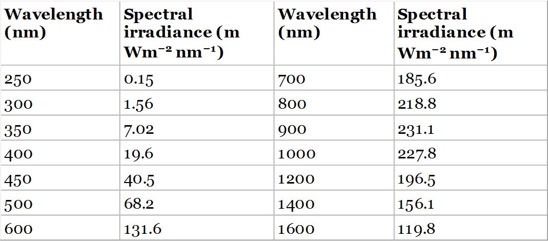
The pyrolytic graphite discs that comprise the cavity are heated electronically, as indicated. Fully calibrated, this is a precision, broadband radiometric source. However, it is not practical for use in a standard laboratory setting. Therefore, practical calibration is generally carried out using transfer standards. These are simpler light sources whose spectral irradiance has been calibrated (ultimately) against a primary source at an NMI. One very commonly used example of a transfer standard is a filament emission lamp or FEL. This lamp is simply a well characterised and calibrated quartz halogen lamp. Generally the FEL is a 1000 W lamp whose irradiance at a nominal distance of 500 mm has been measured and calibrated at an NMI. These emission lamps approximate to a 3200 K blackbody source. Table 7.2 shows calibrated spectral radiance levels for a typical lamp.
The process of transferring the standard from the primary to the transfer standard does increase the uncertainty of the calibration of the FEL lamp and the calibration uncertainty for this type of lamp is of the order of 1–2%, depending upon the wavelength. Any subsequent use of the FEL in laboratory calibration of photodetector sensitivity must faithfully replicate the NMI calibration set up. The laboratory set up might look like that shown in Figure 7.19.
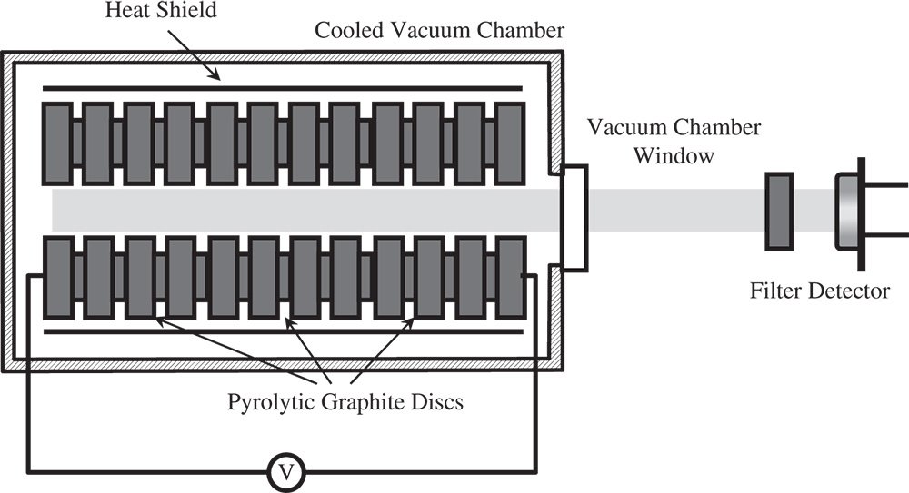
Figure 7.18 Blackbody radiometric source.
Table 7.2 Spectral radiance for typical calibrated FEL lamp.
Great care must be taken to minimise the contribution from scattered light from the surroundings. The original calibration is based entirely on direct radiation from the lamp; any contribution from scattered light would compromise this.
7.6.2.3 Other Calibration Standards
Measurement, characterisation, and modelling of reflection represent an important part of radiometry as the preceding discussions illustrate. Measurement of reflectivity, might be on either polished (specular) or diffuse surfaces. In the former case, the reflectivity is a simple function of the incident angle as, for specular reflection, the reflected angle is pre-determined. For laboratory measurements of specular reflectance, reference standards may be obtained that have been calibrated at NMIs. These might be aluminised mirrors or polished glass blanks with low, but measurable reflectivity. For diffuse reflection, the interest is not only in total reflection (total hemispherical reflectivity) but also in its distribution with angle. In this case, full characterisation of BRDF is of interest. Again, routine laboratory measurements are facilitated by the provision of calibrated artefacts. These might include ∼100% reflectance standards in addition to matt black standards to provide a nominal zero reference.
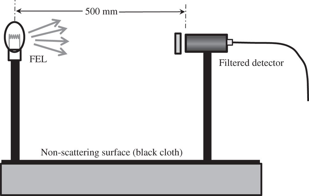
Figure 7.19 FEL lamp calibration.
7.7 Photometry
7.7.1 Introduction
Radiometry is concerned with the measurement of absolute flux levels of optical radiation. However, in many practical instances, we are rather concerned with the effect of these flux levels on detection systems, most notably the human eye. For instance, real, tangible radiometric fluxes in the infrared are of no relevance to human vision. Therefore, photometry is concerned with optical fluxes as mediated by some detection sensitivity, most particularly of the human eye. Naturally most of the discussion here relates to visual photometry, although there are other areas of photometry, such as astronomical photometry.
7.7.2 Photometric Units
For visual photometry, each radiometric unit has its corresponding photometric unit. The photometric equivalent of radiant flux is the luminous flux expressed in lumens and the equivalent of radiant intensity is luminous intensity whose base unit is the candela. Similarly, the radiometric quantities, irradiance and radiance correspond to illuminance and luminance respectively in photometry. The base unit for illuminance is lux and that for luminance is candela per square metre. Units for luminance are occasionally referred to as nits. Comparison of the radiometric and photometric quantities is set out in Table 7.3.
Each photometric quantity is derived from the respective radiometric quantity by integration across the visible spectrum using a spectrally dependent weighting function V(λ). This weighting function is a standardised representation of the sensitivity of the human eye. Normally, this standard weighting function is taken to represent photopic (daytime) vision as opposed to scotopic (dark adapted) vision. This standard weighting function, V(λ), or luminous efficiency function, was originally established by the Commission Internationale de l'Éclairage (CIE) in 1924. By definition, V(λ) has a maximum value of unity and, for the photopic function, this occurs at a wavelength of 555 nm, corresponding to the peak sensitivity of the human eye. The function has since been revised slightly on a number of occasions most notably in 1978 and 2005. Figure 7.20 shows the plot for both photopic and scotopic sensitivity.
Table 7.3 Photometric quantities.
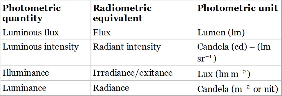
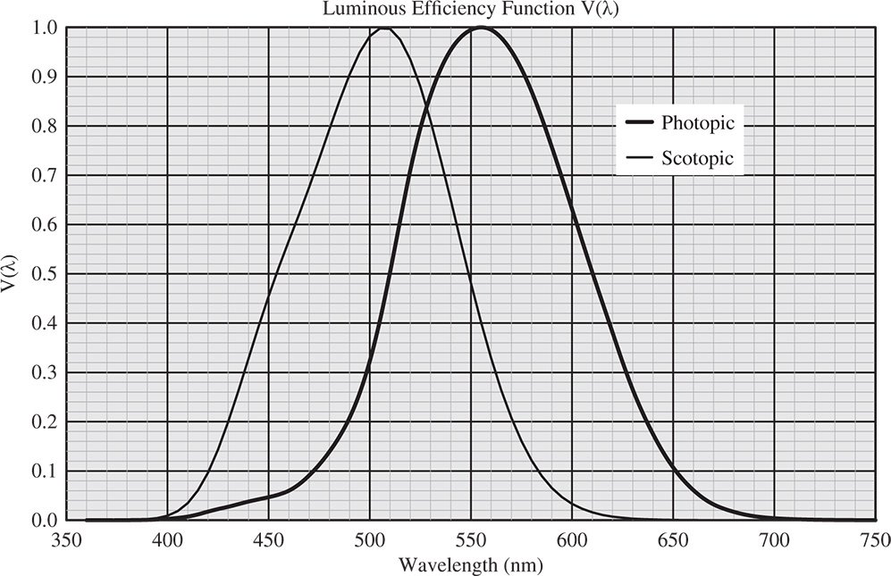
Figure 7.20 Luminous efficiency function.
However, V(λ) is only a relative measurement of luminous efficiency. To link photometric units to their corresponding radiometric quantities a constant of proportionality, KM, must be added to relate the two. That is to say, if the radiometric spectral flux is Φr(λ) and the corresponding luminous flux is Φp(λ) then the two may be linked by the following equation:
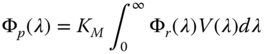
The value of KM is defined as 683.002 lm W−1. That is to say, an optical beam with a wavelength of 555 nm (actually 5.4 × 10¹⁴ Hz or 555.17 nm) and having a luminous flux of 1 lm, actually has a radiant flux of 1/683.002 W. At first sight, this might seem a rather curious definition. The reason for this is essentially historical. It is the candela, rather than the lumen that forms the base SI photometric unit. All other photometric units are derived from the candela. As such, the candela is defined as the luminous intensity of a source of monochromatic radiation of frequency 5.4 × 10¹⁴ Hz having a radiant intensity of 1/683.002 W sr−1. However, originally the definition of luminous intensity was related directly to the output of a standard hydrocarbon burning lamp. In fact, the candela was historically related to an earlier unit of luminous flux, candlepower. So, for historical consistency, a radiometric intensity 1/683 W sr−1 at 555 nm is broadly related to the output of a ‘standard candle’. Attempts were made to produce reference sources of luminous intensity using standard blackbody emitters. However, these proved to be unreliable and were superseded by the current radiometric definition.
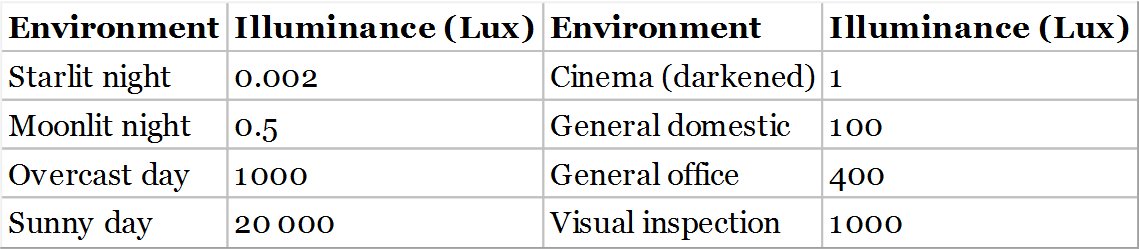
Table 7.4 Typical illuminance levels for difference environments.
7.7.3 Illumination Levels
Since optical photometry is fundamentally connected to light levels as mediated by the sensitivity of the human eye, levels of illuminance are intimately related to the ability to perform visually based tasks. For the indoor environment, lighting levels may be designed for specific areas. A generally comfortable level of illuminance for a domestic environment is around 100 lx. For an office environment, where moderately demanding visual tasks are to be performed, a level of 300–500 lx is acceptable. For more critical tasks, such as visual inspection, a higher level of 500–2000 lx may be called for. Of course, daylight illumination levels are very much higher, ranging from 1000 lx on an overcast day to 25 000 lx for full sunshine. Table 7.4 sets out some typical illumination levels for different environments:
Another important consideration in illumination sources is their efficiency. The efficiency of domestic and industrial light sources is measured in lumens per watt. From that perspective, the ideal light source is a monochromatic source with a wavelength of 555 nm, giving a maximum efficiency of 683 lm W−1 of optical output. A reasonable approximation to this is the sodium vapour street lamp, providing virtually monochromatic light at 589 nm with an electrical efficiency of 200 lm W−1. However, such a highly coloured source is not acceptable for domestic and industrial applications where broadband or nominally ‘white’ sources are preferred. The least efficient sources are incandescent tungsten sources which are being replaced in domestic and industrial applications due to their poor energy efficiency. Their immediate successors, fluorescent mercury lamps create broadband emission from fluorescent phosphor coatings irradiated by ultraviolet emission from mercury spectral lines. More latterly, these are being replaced by white light LEDs which rely on ultraviolet emission from gallium nitride diodes to create broad band fluorescence from phosphors. Efficiencies of these sources are set out in Table 7.5.