


Полная версия
Optical Engineering Science
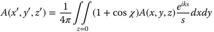
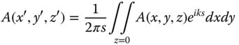
The Kirchoff diffraction formula lacks the generality of the Rayleigh formulae, as it only applies where the secondary wave propagation distance is much greater than the wavelength. However, it provides a useful reference point for comparison with the Huygens approach. The factor, 1 + cosχ is the inclination factor that was alluded to previously. A further approximation may be made where the system is paraxial, i.e. where cosχ ∼ 1. In this case, there is no inclination factor to speak of. Furthermore, if the axial displacement s is very much larger than the lateral extent of the illuminated area defined by A(x, y, z), then for all intents and purposes, s is constant and the inverse term may be taken outside the integral. This is the so-called Fraunhofer approximation and may be written as:
6.4 Diffraction in the Fraunhofer Approximation
The assumptions underlying the Fraunhofer approximation are relevant to a wealth of problems in optical engineering. In particular, the approximation relates the behaviour and distribution of electromagnetic radiation in two distinct zones, the so-called near field and far field. Separation of these two zones must be such that the preceding approximations apply, i.e. that the axial displacement is much larger than the lateral extent of the radiation field and, of course, is much greater than the wavelength. We now wish to calculate the amplitude on a sphere whose vertex is located at z′ = z0 and whose centre is located at z = 0, where the near field is located. Figure 6.4 shows the general scheme.
Choice of the reference sphere centred on the near field location places the following constraint upon the variables, x, y, x′, y′, and z′:
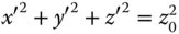
Expanding the propagation distance, s, in terms of the variables, x, y, and x′, y′ we can re-write Eq. (6.11):

In the Fraunhofer approximation, we are seeking to calculate the amplitude at the limit where z0 tends to infinity. We wish to know the far field distribution at some angle, θ, where z0 tends to infinity. Therefore, we can assume that x′ ≫ x and y′ ≫ y. Hence, the diffraction formula may be recast in the following form:
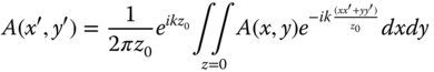
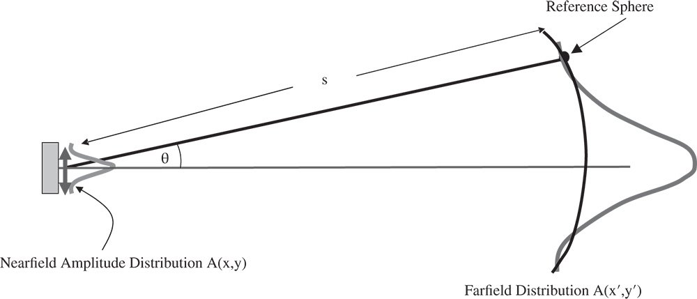
Figure 6.4 Far field diffraction.
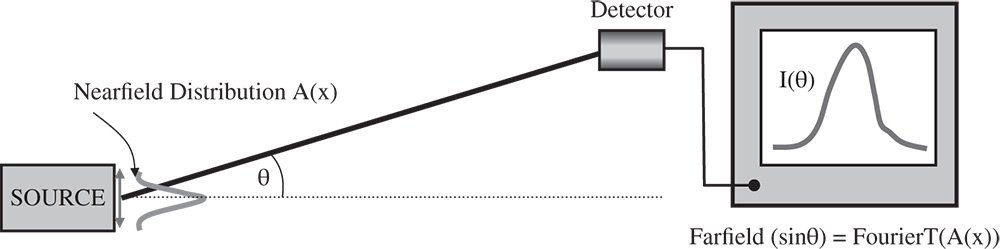
Figure 6.5 Far field diffraction of laser beam emerging from fibre.
Equation (6.12) has the form of a Fourier transform. So, the far field diffraction pattern of a near field amplitude distribution is simply given by the Fourier transform of that near field distribution. Of course, we must understand all the caveats that apply to this treatment, namely that the far field distribution must imply that the distance of the ‘far field’ location from the near field location must be sufficiently great. Finally, we might like to cast Eq. (6.12) more conveniently in terms of the angles involved:
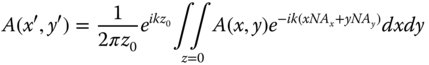
NAx and NAy are the numerical apertures (sine of the angles) in the x and y directions respectively.
A typical example of the application of Fraunhofer diffraction might be the emergence of a laser beam from a very small, single mode optical fibre a few microns across. As the beam emerges from the fibre, it will have some near field distribution. In fact, the spatial variation of this amplitude may be approximated by a Gaussian distribution. In the light of the previous analysis, the angular distribution of the emitted radiation far from the fibre will be the Fourier transform of the near field distribution. This is shown in Figure 6.5.
We will be returning to the subject of diffraction and laser beam propagation later in this chapter. A more traditional concern is the impact of diffraction upon image formation in real systems. As far as the design of optical systems is concerned, hitherto we have only been concerned with the impact of aberrations in limiting optical performance. In the next section, we will examine the application of Fraunhofer diffraction to the study of image formation in optical system and the way in which the presence of diffraction limits optical resolution.
6.5 Diffraction in an Optical System – the Airy Disc
In the Fraunhofer approximation, we considered the effect of diffraction by considering a near field amplitude distribution and a far field, nominally located at infinity. However, it is not necessary for the far field to be physically located at infinity. For example the (second) focal point of an optical system is conjugated to an object plane located at infinity. In this instance, the relation of the two planes is perfectly described by the Fraunhofer approximation. This is illustrated schematically in Figure 6.6 which shows the realisation of the far field of a laser source. The focus of the lens in Figure 6.6 is conjugate to infinity in object space and, assuming the lens aberration is not significant, then the Fraunhofer diffraction pattern would be imaged at this location.
In the case of the near field distribution associated with the laser, the far field distribution will be given by the Fourier transform of the near field distribution, but mediated by the focal length of the lens. In other words, the spatial distribution, A(x′, y′) of the far field at the lens focus is given by:
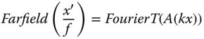
In practice, the quantity, x′/f, can be regarded as equivalent to the numerical aperture (NA) associated with the far field distribution.
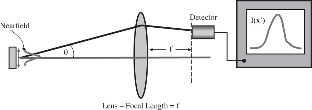
Figure 6.6 Imaging of a Fraunhofer diffraction pattern by a simple lens.
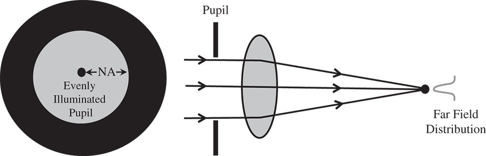
Figure 6.7 Diffraction of evenly illuminated pupil.
In terms of a real optical system, the greatest practical interest is invested in the diffraction produced by the pupil. For an object located at infinity and the physical stop located in object space, the far field diffraction pattern of the pupil will be formed at the focal point of the system. Of course, the pupil, or its image, the exit pupil, is of great significance in the analysis of an optical system as the system optical path difference (OPD) is, by convention, referenced to a sphere whose vertex lies at the exit pupil. As such, the diffraction pattern produced by a uniformly illuminated circular disc is of prime importance in the analysis of optical systems.
We will now assume that an optical system is seeking to image a point object, and the exit pupil size can be expressed as an even cone of light with a numerical aperture, NA. It will produce a diffraction pattern at the focus of the system, whose extent and form we wish to elucidate. A schematic of this scenario is shown in Figure 6.7.
We are now simply required to determine the Fourier transform of a circular disc. In fact, the Fourier transform of a circular disc is described in terms of J1(x), a Bessel function of the first kind. Proceeding along the lines set out in Eq. (6.14), we find that the far field distribution at the system focus is given by:
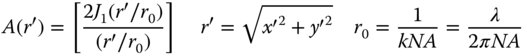
It is natural, of course, that the far field distribution retains the circular symmetry of the near field. We have to remember that, in this analysis, we have calculated the amplitude (electric field) of the far field distribution. The flux density, I(r′), is proportional to the square of the electric field and this is given by:
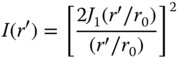
The pattern produced at the far field location, as defined by Eq. (6.16) is known as the Airy disc. For r′ → 0, Eq. (6.16) tends to one. Thus, all values computed by Eq. (6.16) represent the local flux taken in ratio to the central maximum. The form of the Airy disc consists of a bright central region surrounded by a number of weaker rings. This is shown in Figure 6.8.
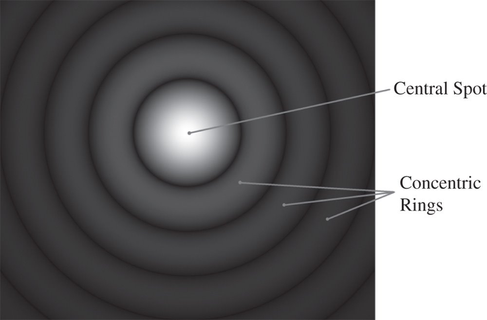
Figure 6.8 Airy disc.
The importance of the Airy disc lies in the fact that it represents the ideal replication of a point source in a totally unaberrated system. Hitherto, in the idealised geometrical optics representation, a point source would be replicated as a point image. The presence of diffraction, therefore, critically compromises resolution. That is to say, even in a perfect optical system, the lateral resolution of the system is limited by the extent of the Airy disc. At this point it is useful to examine the form of the Airy disc in more detail. Figure 6.9 shows a graphical trace of the Airy disc, expressed in terms of the ratio r′/r0.
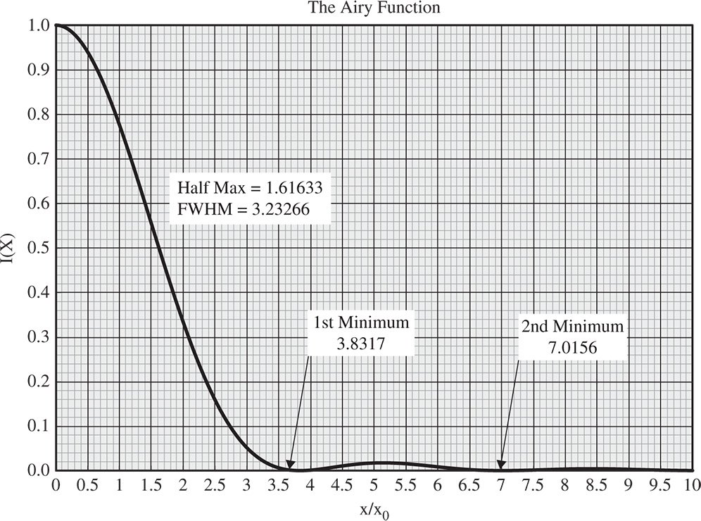
Figure 6.9 Graphical trace of Airy disc.
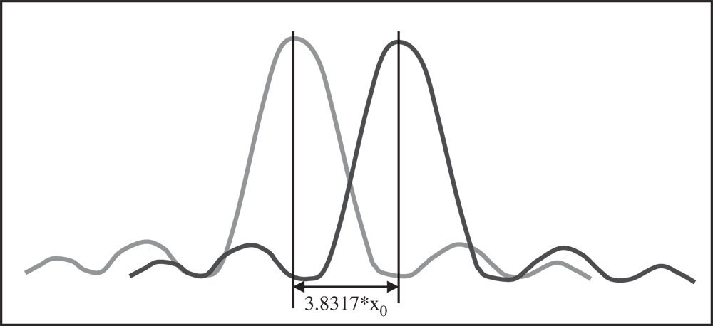
Figure 6.10 The Rayleigh criterion and ideal diffraction limited resolution.
As illustrated in Figure 6.9, the full width half maximum (FWHM) is equal to 3.233r0. Equally significant is the presence of local minima at 3.832r0 and 7.016r0. It is more informative to express these values in terms of the wavelength and numerical aperture. This gives the FWHM as 0.514λ/NA and the locations of the minima as 0.610λ/NA and 1.117λ/NA. At first sight, the FWHM may seem a useful indication of the ideal optical system resolution. In practice, it is the location of the first minimum that forms the basis for the conventional definition of ideal resolution. The rationale for this is shown in Figure 6.10.
Considering two adjacent point sources, these are said to be resolved when the maximum of one Airy disc lies at the minimum of the other. Therefore the separation of the two images must be equal to 0.610λ/NA. This is the so-called Rayleigh criterion for diffraction limited imaging. Under the Rayleigh criterion, two separated and resolved peaks are seen with a local minimum between them at 73.5% of the maximum. This is illustrated in Figure 6.11
At this point, we will re-iterate the formula describing diffraction limited resolution under the Rayleigh criterion, as it is fundamental to the enumeration of resolution in a perfect optical system. This is set out in Eq. (6.17).
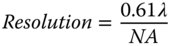
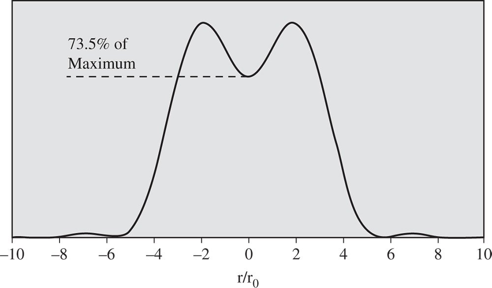
Figure 6.11 Profile of two point sources just resolved under Rayleigh criterion.
Worked Example 6.1 Microscope Objective
A microscope objective has a numerical aperture of 0.8. What is the diffraction limited resolution at the D wavelength of 589.3 nm?
Calculation is very straightforward, we simply need to substitute the relevant values into Eq. (6.17).
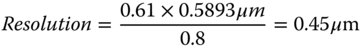
The resolution is 0.45 μm.
This figure only applies to ‘perfect’ or diffraction limited in an aberration-free system. The presence of aberrations will affect the resolution, as will be considered in the next section.
6.6 The Impact of Aberration on System Resolution
6.6.1 The Strehl Ratio
In the preceding analysis we examined the diffraction pattern produced by a circular disc – namely the pupil. This produced the Airy diffraction pattern. In this analysis, we ignored the impact of phase, i.e. the possibility that the amplitude across the pupil might have a complex component. In fact, for a point source, the phase across the pupil is, by definition, directly related to the OPD. That is to say, if we assume that the modulus of the near field amplitude, A(x, y) is unity, the complex amplitude is given by:

where Φ(x, y) is the wavefront error across the pupil.
The final diffraction pattern is given by the Fourier transform of the above which, from Eq. (6.13), is given by:
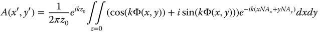
We now wish to compute the amplitude at the central location of the far field pattern, i.e. where NAx and Nay = 0. In this case the Fourier transform can be further simplified:
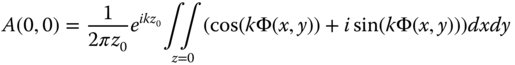
For an optical system that is close to perfection, or almost diffraction limited, we can make the further assumption that kΦ ≪ 1 at all locations across the pupil. We find that the ratio of the amplitude with the presence of aberration to that without is approximately given by:
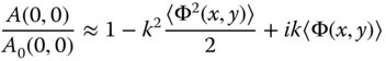
The expressions in the pointed brackets in Eq. 6.19 represent the mean square wavefront error and the mean wavefront error respectively.
However, the expression in Eq. (6.20) is merely the amplitude of the disturbance and not the flux. To calculate the flux density at the centre of the diffraction pattern, we need to multiply Eq. (6.19) by its complex conjugate. This gives:
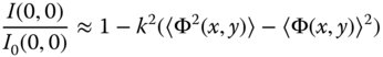
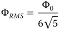
The expression contained within the brackets is merely the variance of the wavefront error taken across the pupil. If we define the root mean square (rms) wavefront error, Φrms, as the rms value computed under the assumption that the average wavefront error has been normalised to zero, we get the following fundamental relationship:
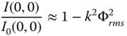
Equation (6.22) is of great significance. The ratio expressed in Eq. (6.22), the ratio of the aberrated and unaberrated flux density, is referred to as the Strehl ratio. The Strehl ratio is a measure of the degradation produced by the introduction of system imperfections. Of course, Eq. (6.22) only applies where kΦ2rms ≪ 1. The fact that the peak flux of a diffraction pattern is reduced by the introduction of aberration necessarily implies that the distribution is in someway broadened, i.e. the resolution is reduced. For example, if the Strehl ratio is 0.8, then the area associated with the diffraction pattern is likely to have increased by about 20% and the linear dimension by about 10%.
6.6.2 The Maréchal Criterion
The Strehl ratio is of great practical significance. It affords a useful, practical, but somewhat arbitrary definition of ‘diffraction limited’ imaging. Where the Strehl ratio is 0.8 or greater, the image is said to be diffraction limited. This is the so-called Maréchal criterion. It can be expressed as follows:
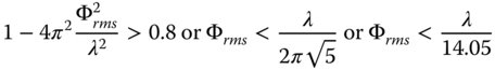
This condition is widely accepted as the basis for the definition of diffraction limited imaging. As a measure of system wavefront error, the peak to valley wavefront error, Φpv ≪ λ/4 is often preferred, in practice. This is very much a traditional description of system wavefront error, preserved for historical reasons, primarily on account of the ease of reckoning peak to valley fringe displacements on visual images of interferograms. This consideration has, of course, been displaced by the ubiquitous presence of computer-based interferometry which has rendered the calculation of rms wavefront errors a trivial process. Nonetheless, the peak to valley description remains prevalent. Although dependent upon the precise distribution of wavefront error, as a rule of thumb, the peak to valley wavefront error is about 3.5 times the standard deviation or rms value. Therefore, we can set out another condition for diffraction limited imaging.

Worked Example 6.2 A simple ×10 microscope objective is to be made from a BK7 plano-convex lens and is to operate at the single wavelength of 589.3 nm. The refractive index of BK7 at 589.3 nm is 1.518 and the assumed microscope tube length is 160 mm. We also assume that only the microscope objective contributes to system aberration. What is the maximum objective numerical aperture consistent with diffraction limited performance, assuming on-axis spherical aberration as the dominant aberration?
Firstly, for a wavelength of 589.3 nm, from Eq. (6.22):

For a ×10 objective, the focal length should be 160/10 = 16 mm for a 160 mm tube length. The tube length is much longer than the objective focal length, so, for all intents and purposes, the image is at the infinite conjugate, as illustrated.
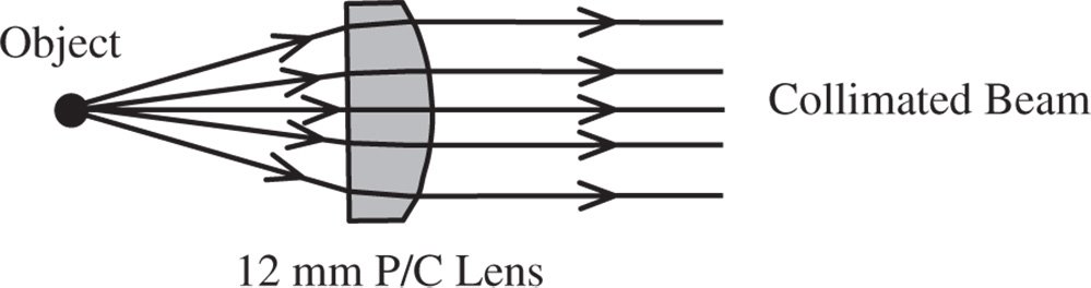
Note that the curved surface faces the infinite conjugate in order to minimise spherical aberration. Thus, in this instance, the conjugate parameter is 1 and the lens shape factor is −1. From Eq. (4.30a)
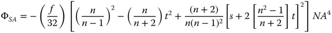
Substituting the values of s and t:
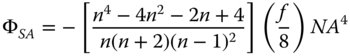
Substituting the values of n (1.518) and f (16 mm) into the equation, we get:
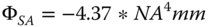
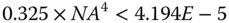
Further assuming that we are using defocus to ‘balance’ and minimise aberrations, we can relate the rms wavefront error to the maximum OPD:

For the ‘diffraction limited’ condition to be fulfilled the rms wavefront error must be less than 41.94 nm.
The minimum numerical aperture is thus 0.107. Substituting this value into Eq. (5.17), then it is clear that the resolution of the objective is 3.37 μm. The design of complex objectives does, of course, generally proceed by virtue of ray tracing. However, this illustration does provide some insight into the limitations of simple optics and the value added by more complex designs.
6.6.3 The Huygens Point Spread Function
The Huygens point spread function is the diffraction pattern produced in the image plane by a point source located at the object plane. Determination of the point spread function proceeds as per Eq. (6.18) and so is fundamentally influenced by the system wavefront error across the pupil. Of course, as previously argued, any wavefront error reduces the flux at the axial location in proportion to the Strehl ratio. In concert with this, the width of the diffraction pattern increases with increasing wavefront error.
As will be discussed in more detail later, where the wavefront error is small, purely geometrical ray tracing produces a very different spatial distribution when compared to the point spread function. Naturally, in the limit where the wavefront error becomes large, the Huygens point spread function tends to the geometrical spot distribution. This is quite an important consideration, as it impacts how optical systems are optimised with regard to optical performance. If the intention is to design a diffraction limited system, the most efficient optimisation proceeds by minimising the wavefront error. However, where the intended wavefront error is large when compared to the diffraction limit, it is best to optimise the system by minimising the geometrical spot size.
6.7 Laser Beam Propagation
6.7.1 Far Field Diffraction of a Gaussian Laser Beam
The far field divergence of a laser beam may be accounted for by the Fraunhofer approximation according to Eq. (6.13). In the treatment of a laser beam, we consider the beam to have a ‘near field’ location, or beam waist, where the phase is uniform across a plane perpendicular to the propagation direction. That is to say, the wavefronts are planar at this beam waist location. In addition, it must be assumed that the wavefront is ‘coherent’, i.e. that an unambiguous phase relation exists across the wavefront at all times. We now wish to know the disturbance produced by this near field distribution in the far field. To make the problem tractable, we assume that the near field distribution of the laser beam waist may be described by a Gaussian function. This is a useful approximation, however, it must be emphasised that this is an approximation. In practice, the profile of a laser beam is not quite Gaussian, with more flux being in the wings, far from the centre, than would be expected from a Gaussian distribution.
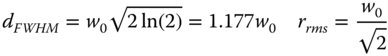
In the Gaussian approximation, we may, for example, describe the laser beam emerging from the end of a single mode fibre or from the output of a semiconductor laser facet or from a helium neon laser. The size of the beam waist is described by the parameter, w0, namely the radial distance at which the amplitude, A(r), falls to 1/e, or 37% of the peak value. When expressed in terms of flux, the size of the beam waist, r0 defines the radius at which the flux, I(r) falls to (1/e)2 or 13% of the peak value. For example, in the case of a single mode telecoms fibre, a laser beam emerging from the end of the fibre might have a beam waist, w0 of 5.5 μm. Equation (6.25) expresses the form of the laser beam profile:

Having characterised the beam waist in this way, it is useful to relative it to both the FWHM, dFWHM, and the rms radius, rrms.
In the Fraunhofer approximation, the far field may be derived from the Fourier transform of the near field. At this point, the significance of the Gaussian representation becomes clear, as the Fourier transform of a Gaussian is another Gaussian. The far field representation is thus given by another Gaussian, with the divergence expressed by a characteristic numerical aperture, NA0.

From the Fourier transform, it is possible to derive a clear relationship between the near field beam waist, w0, and the far field divergence, NA0. This is given by Eq. (6.28).
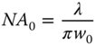
As one might expect, the far field divergence is inversely proportional to the size of the beam waist, a smaller beam waist effecting a larger divergence.