

Полная версия
Optical Engineering Science
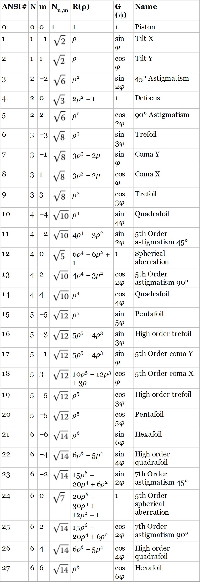
Table 5.2 First 28 Zernike polynomials.

The rms wavefront error has thus been reduced by a factor of six by the focus compensation process. Furthermore, this analysis feeds in to the discussion in Chapter 3 on the use of balancing aberrations to minimise wavefront error. For example, if we have succeeded in eliminating third order spherical aberration and are presented with residual fifth order spherical aberration, we can minimise the rms wavefront error by balancing this aberration with a small amount of third order aberration in addition to defocus. Analysis using Zernike polynomials is extremely useful in resolving this problem:

As previously outlined, the uncompensated rms wavefront error may be calculated from the RSS sum of all the four Zernike terms. Naturally, for the compensated system, we need only consider the first term.
(5.24)

For the fifth order spherical aberration, the rms wavefront error has been reduced by a factor of 20 through the process of aberration balancing. In terms of the practical application of this process, one might wish to optimise an optical design by minimising the rms wavefront error. Although, in practice, the process of optimisation will be carried out using software tools, nonetheless, it is useful to recognise some key features of an optimised design. By virtue of the previous example, optimisation of spherical aberration should lead to an OPD profile that is close to the 5th order Zernike term. This is shown in Figure 5.5 which illustrates the profile of an optimised OPD based entirely on the relevant fifth order Zernike term. The graph plots the nominal OPD again the normalised pupil function with the form given by the Zernike polynomial, n = 6, m = 0.
In the optimisation of an optical design it is important to understand the form of the OPD fan displayed in Figure 5.5 in order recognise the desired endpoint of the optimisation process. It displays three minima and two maxima (or vice versa), whereas the unoptimised OPD fan has one fewer maximum and minimum. Thus, although the design optimisation process itself might be computer based, nevertheless, understanding and recognising the how the process works and its end goal will be of great practical use. That is to say, as the computer-based optimisation proceeds, on might expect the OPD fan to acquire a greater number of maxima and minima.
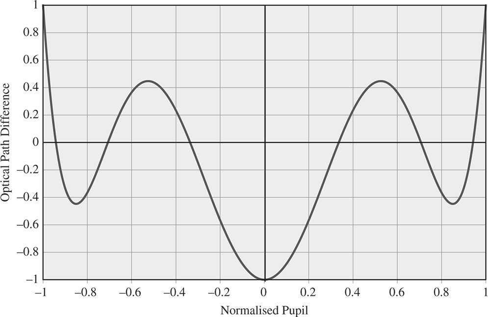
Figure 5.5 Fifth order Zernike polynomial and aberration balancing.
One can apply the same analysis to all the Gauss-Seidel aberrations and calculate its associated rms wavefront error.
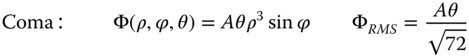
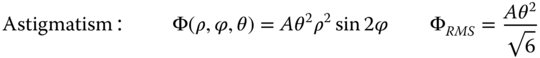
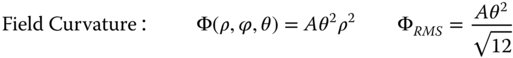
θ represents the field angle
Equations (5.25a)–(5.25d) are of great significance in the analysis of image quality, as the rms wavefront error is a key parameter in the description of the optical quality of a system. This will be discussed in more detail in the next chapter.
Worked Example 5.2 A plano-convex lens, with a focal length of 100 mm is used to focus a collimated beam; the refractive index of the lens material is 1.52. It is assumed that the curved surface faces the infinite conjugate. The pupil diameter is 12.5 mm and the aperture is situated at the lens. What is the rms spherical aberration produced by this lens – (i) at the paraxial focus; (ii) at the compensated focus? What is the rms coma for a similar collimated beam with a field angle of one degree?
Firstly, we calculate the spherical aberration of the single lens. With the object at infinity and the image at the first focal point, the conjugate parameter, t, is equal to −1. The shape parameter, s, for the plano convex lens is equal to 1 since the curved surface is facing the object. From Eq. (4.30a) the spherical aberration of the lens is given by:
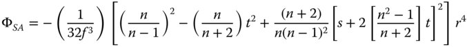
rmax = 6.25 mm (12.5/2); f = 100 mm; n = 1.52; s = 1; t = −1
By substituting these values into the above equation, the spherical aberration may be directly calculated:

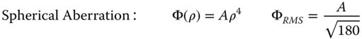
where A = 4.13 × 10⁻⁴ mm ρ = r/rmax
From Eq. (5.23), the uncompensated rms wavefront error is A/√5 and the compensated error is A/√180. Therefore the rms values are given by:
Φrms(paraxial) = 185 nm; Φrms(compensated) = 30.8 nm
Secondly, we calculate the coma. From (4.30b), the coma of the lens is given by:
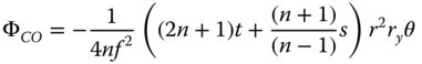
Again, substituting the relevant values for f, n, rmax, s, and t, we get:
where A = 3.24 × 10⁻³ mm ρ = r/rmax ry = r sin ϕ
From (5.25b)

We are told that θ = 1° or 0.0174 rad. Therefore, Φrms = 6.66 × 10⁻⁶or 6.66 nm
5.3.4 General Representation of Wavefront Error
We have emphasised the synergy between Zernike polynomials and the classical treatment of aberrations in an axially symmetric optical system, i.e. the Gauss-Seidel aberrations. However, in practice, in real optical systems, these axial symmetries are often compromised, either by accident or by design. Some systems are deliberately designed whereby not all optical surfaces are aligned to a common axis. These will inevitably introduce non-standard wavefront aberrations into the system. Most significantly, even with a symmetrical design, component manufacturing errors and system alignment may introduce more complex wavefront errors into the system. Naturally, alignment errors create an off-axis optical system ‘by accident’. Manufacturing or polishing errors might produce an optical surface whose shape departs from that of an ideal sphere or conic in a somewhat complex fashion. For example, the effects of these errors may be to introduce a trefoil term (n = 3, m = 3) into the wavefront error; this is not a standard Gauss-Seidel term.
As argued, Zernike polynomials are widely used in the analysis of wavefront error both in the design and testing of optical systems. From a strictly analytical and theoretical point of view the description of wavefront error in terms of its rms value is the most meaningful. However, for largely historical reasons, wavefront error is often presented as a ‘peak to valley’ error. That is to say, the value presented is the difference between the maximum and minimum OPD across the pupil. Historically, the wavefront error for a system might have been derived from a visual inspection of a fringe pattern in an interferogram. The maximum deviation of fringes is relatively straightforward to estimate visually from a fringe pattern which might have been produced photographically. However, the rms wavefront error is more directly related to system performance. Calculation of the rms wavefront error across a pupil is a mathematical process that requires computational data acquisition and analysis and has only been universally available in more recent times. Therefore, the use of the peak to valley description still persists.
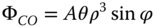
One particular disadvantage of the peak to valley description is that it is unusually responsive to large, but highly localised excursions in the wavefront error. More generally, as a rule of thumb, the peak to valley is considered to be 3.5 times the rms value. Of course, this does depend upon the form of the wavefront error. Table 5.3 sets out this relationship for the first 11 Zernike terms (apart from piston). For comparison, a standard statistical measure is also presented – namely for a normally distributed wavefront error profile, the limits containing 95% of the wavefront error distribution (±1.96 standard deviations).
The values presented in Table 5.3 are simply the ratio of the peak to valley (p-to-v) error for that particular distribution. To overcome the principal objection to the p-to-v measure, namely its heightened sensitivity to local variation a new peak to valley measure has been proposed by the Zygo Corporation. This measure is known as P to Vr or peak to valley robust. In this measure, the wavefront error is fitted to a set of 36 Zernike polynomials. Although this process is carried out by computational analysis, the procedure is very simple. Essentially the calculation process exploits the orthonormal properties of the polynomial set and calculates the contribution of each Zernike term using the relation set out in Eq. (5.12). Following this process, the maximum and minimum of the fitted surface is calculated and the revised peak to valley figure calculated. Of course, the reduced set of 36 polynomials cannot possibly replicate localised asperities with a high spatial frequency content. Therefore, the fitted surface is effectively a smoothed version of the original and the peak to valley value derived is more representative of the underlying physics.
Table 5.3 Peak to valley: Root mean square (rms) ratios for different wavefront error forms.
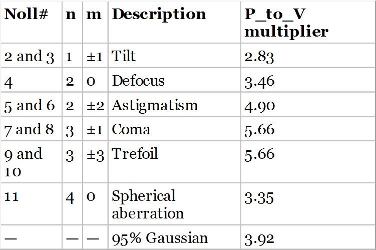
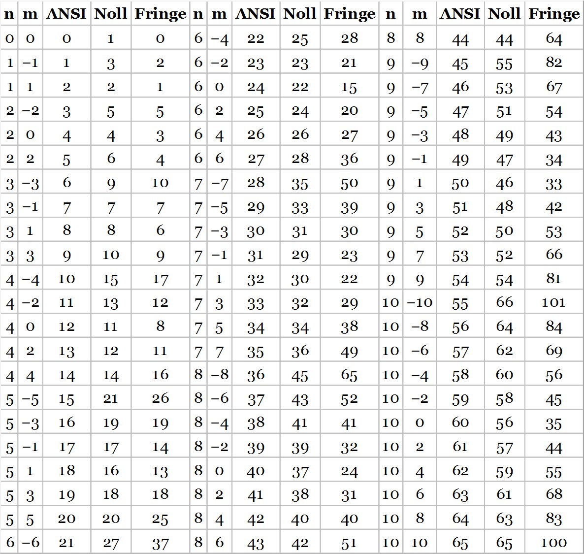
Table 5.4 Comparison of Zernike numbering systems.
It must be stated, at this point, that the 36 polynomials used, in this instance, are not those that would be ordered as in Table 5.1. That is to say, they are not the first 36 ANSI standard polynomials. As mentioned earlier, there are, unfortunately, a number of competing conventions for the numbering of Zernike polynomials. The convention used in determining the P to Vr figure is the so called Zernike Fringe polynomial convention. The logic of ordering the polynomials in a different way is that this better reflects, in the case of the fringe polynomial set, the spatial frequency content of the polynomial and its practical significance in real optical systems.
5.3.5 Other Zernike Numbering Conventions
The ordering convention adopted by the Fringe polynomials expresses, to a significant degree, the spatial frequency content of the polynomial. As a consequence, the polynomials are ordered by the sum of their radial and polar orders, rather than primarily by the radial order. That is to say, the polynomials are ordered by the sum n + m, as opposed to n alone. For polynomials of equal ‘fringe order’ they are then ordered by descending values of the modulus of m, i.e. |m|, with the positive or cosine term presented first.
Another convention that is very widely used is the Noll convention. The Noll convention proceeds in a broadly similar way to the ANSI convention, in that it uses the radial order, n, as the primary parameter for sorting. However, there are a number of key differences. Firstly, the sequence starts with the number one, as opposed to zero, as is the case for the other conventions. Secondly, the ordering convention for the polar order, m, as in the case of the fringe polynomials, follows the modulus of m rather its absolute value. However, the ordering is in ascending sequence of |m|, unlike the fringe polynomials. The ordering of the sine and cosine terms is presented in such a way that all positive m (cosine terms) are allocated an even number. In consequence, sometimes the sine term occurs before the cosine term in the sequence and sometimes after. Table 5.4 shows a comparison of the different numbering systems up to ANSI number 65.
Further Reading
American National Standards Institute (2017). Methods for Reporting Optical Aberrations of Eyes, ANSI Z80.28:2017. Washington DC: ANSI.
Born, M. and Wolf, E. (1999). Principles of Optics, 7e. Cambridge: Cambridge University Press. ISBN: 0-521-642221.
Fischer, R.E., Tadic-Galeb, B., and Yoder, P.R. (2008). Optical System Design, 2e. Bellingham: SPIE. ISBN: 978-0-8194-6785-0.
Hecht, E. (2017). Optics, 5e. Harlow: Pearson Education. ISBN: 978-0-1339-7722-6.
Noll, R. (1976). Zernike polynomials and atmospheric turbulence. J. Opt. Soc. Am. 66 (3): 207.
Zernike, F. (1934). Beugungstheorie des Schneidenverfahrens und Seiner Verbesserten Form, der Phasenkontrastmethode. Physica 1 (8): 689.
6
Diffraction, Physical Optics, and Image Quality
6.1 Introduction
Hitherto, we have presented optics purely in terms of the geometrical interpretation provided by the propagation and tracing of rays. Notwithstanding this rather simplistic foundation, this conveniently simple picture is ultimately derived from an understanding of the wave nature of light. More specifically, Fermat's principle, which underpins geometrical optics is itself ultimately derived from Maxwell's famous wave equations, as introduced in Chapter 1. However, in this chapter, we shall focus on the circumstances where the assumptions underlying geometrical optics breakdown and this convenient formulation is no longer tractable. Under these circumstances, we must look to another approach, more explicitly tied to the wave nature of light, the study of physical optics. To look at this a little more closely, we must further examine Maxwell's equations. The ubiquitous vector form in which Maxwell's equations are now cast is actually due to Oliver Heaviside and these are set out below:


D, B, E, H, and J are all vector quantities, where D is the electric displacement, B the magnetic field, E the electric field, H the magnetic field strength and J the current density.
The quantities D and E and B and H are themselves interrelated:
The quantities, ε0 and μ0, are the permittivity and magnetic permeability of free space respectively. These quantities are associated specifically with free-space (vacuum). The quantities ε and μ are the relative permittivity and relative permeability of a specific medium or substance.
These equations may be greatly simplified if we assume that the local current and charge density is zero and we are ultimately presented with the classical wave equation.

The next stage in this critique of geometrical optics is to use Maxwell's equation to derive the Eikonal equation, that was briefly introduced in Chapter 1.
6.2 The Eikonal Equation
In Eq. 6.3, we have presented that wave equation in its true vector format. That is to say, the equation describes the electric field, E, as a vector quantity. However, much of what we will present in this chapter is a simplification of the wave equation, known as scalar theory. In this case, it is assumed that the electric field may be represented as a pseudo-scalar quantity. That is to say, the electric field, although varying in magnitude, is confined to one specific orientation and may be treated as if it were a scalar quantity. In fact, this approximation is reasonable where light is closely confined to some axis of propagation, i.e. consistent with the paraxial approximation. Thus, we are to understand that there are some limitations to this treatment.
In presenting the Eikonal equation according the scalar view, we assume that solutions to the wave equation are of the form:
E0(x, y, z) is a slowly varying envelope function and S(x, y, z) is the spatially varying phase of the wave. In fact S(x, y, z) has dimensions of length and when it is equal to the wavelength the phase term it describes is equal to 2π. The angular frequency is denoted by ω and the spatial frequency by k.
The scalar form of the wave equation may be written as
From the above, we can derive the Eikonal equation, but we must assume the E0(x, y, z) and the first differential of S(x, y, z) vary slowly with respect to position. The classical Eikonal equation is set out in Eq. 6.5.
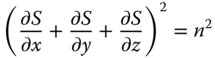
It is clear that by differentiating Eq. (6.4) twice with respect to x, y, and z, that in deriving Eq. (6.5), we are neglecting terms containing the second differential with respect to S. We are also ignoring changes in the envelope function. Thus it is clear that in deriving Eq. (6.5), we are making the following assumptions:
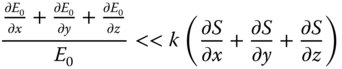
and
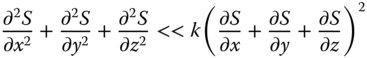
What Eq. (6.6a) suggests is that the envelope function must vary slowly compared to the wavelength. In addition, Eq. (6.6b) suggests that the curvature of the wavefront must be small when compared to the spatial frequency, k. In other words, the assumptions underlying the Eikonal equation are only justified where the radius of any wavefront is much greater than the wavelength. As the Eikonal equation underpins geometrical optics, this sets the limits on the applicability of this methodology, and we must then seek other, more general, means to describe the behaviour of light. These methods are, of course, based on a more rigorous application of Maxwell's equations and are generally categorised under the heading of physical optics.
6.3 Huygens Wavelets and the Diffraction Formulae
Although Maxwell's equations form the rigorous description of electromagnetic wave propagation, we will first proceed from the rather more intuitive description by Huygens' principle. Huygens' principle states that, given a known wave disturbance described by a continuous surface of equal phase – the wavefront, then the amplitude of the wave at any point in space may be determined as the sum of the amplitude of forward propagating wavelets from that surface. This is illustrated in Figure 6.1.
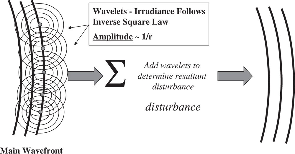
Figure 6.1 Conceptual illustration of Huygens' principle.
The amplitude of the wave represents the strength of the local electric or magnetic field. In this case, in our scalar representation, we consider the amplitude as the magnitude of the vector electric field. The flux or power per unit area transmitted by the wave is determined by the Poynting vector, which is the cross product of the electric and magnetic fields. In the context of this scalar treatment, the flux density is proportional to the square of the electric field. In the Huygens' representation, as illustrated in Figure 6.1, the amplitude of the secondary waves emerging from some point on the original wavefront is inversely proportional to the distance from that point. It follows, therefore, that the flux density associated with that secondary wave follows an inverse square dependence with distance. This is further illustrated in Figure 6.2 which summarises the geometry.
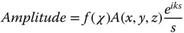
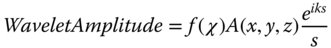
Figure 6.2 describes the contribution to the wave amplitude at point P′ made by a single point, P, on the original wavefront. The original wavefront has an amplitude, A(x, y, z) which may be complex. The angle, χ, is the angle the line from P to P′ makes to the normal to the wavefront. As indicated in Figure 6.2, there is some dependence of the secondary wave amplitude upon this angle, in the form of f(χ). There is no intuitive process that can shed further light on the precise form of this function. Elucidation of this can only be provided by a proper application of Maxwell's equation. Re-iterating the description of the Huygens' representation in Figure 6.2, it can be described more formally, as in Eq. (6.7).
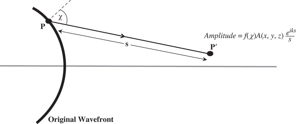
Figure 6.2 Huygens secondary wave geometry.
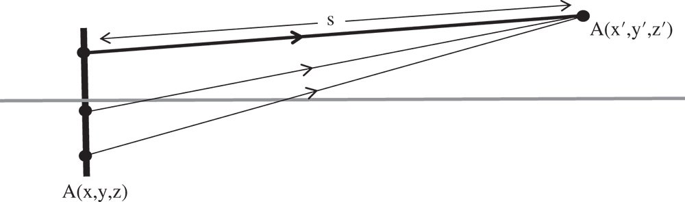
Figure 6.3 Geometry for Rayleigh diffraction equation of the first kind.
Proper application of Maxwell's equations gives rise to a series of equations that are similar in form to the Huygens' representation shown in Eq. (6.7). These include the so-called Rayleigh diffraction formulae of the first and second kinds. In the first case, it is assumed that the amplitude of the wave disturbance A(x, y, z) is known across some semi-infinite plane. We now seek to determine the amplitude, A(x′, y′, z′) at some other point in space. The geometry of this is illustrated in Figure 6.3.
Equation (6.8) shows the Rayleigh diffraction formula of the first kind.
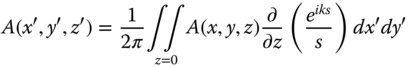
Equation (6.8) is referred to as the Rayleigh diffraction formula of the first kind. In form, Eq. (6.8) is very similar to what one might expect from the summation of an expression of the form shown in the Huygens' representation in Eq. (6.7). We have formally expressed the summation of the Huygens wavelets as a surface integral over the plane, as shown in Figure 6.3. Note, however, instead of the decay of the wavelet amplitude with distance being expressed as in Eq. (6.7), a differential with respect to the axial distance is added. This is crucial, since it gives an insight into the formulation of the inclination term f(χ) which will be explored further a little later.
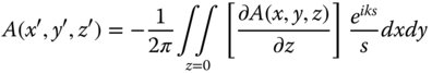
The other condition covered by the Rayleigh formulae occurs where the axial gradient of the amplitude is known rather than the amplitude itself. In this instance, we have the Rayleigh diffraction formula of the second kind.
If we combine these two solutions and make the qualifying assumption that k ≫ 1/s, then we obtain the so-called Kirchoff diffraction formula, which is replicated in Eq. (6.10).