

Полная версия
Optical Engineering Science
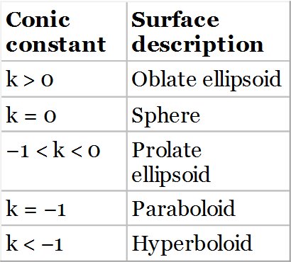
Without the further addition of the even polynomial coefficients, αn, the surfaces are pure conics. Historically, the paraboloid, as a parabolic mirror shape, has found application as an objective in reflective telescopes. As will be seen subsequently, use of a parabolic mirror shape entirely eliminates spherical aberration for the infinite conjugate. The introduction of the even aspheric terms add further useful variables in optimisation of a design. However, this flexibility comes at the cost of an increase in manufacturing complexity and cost. Strictly speaking, at the first approximation, the terms, α1 and α2 are redundant for a general conic shape. Adding the conic term, k, to the surface prescription and optimising effectively allows local correction of the wavefront to the fourth order in r. In this context, the first two even polynomial terms are, to a significant degree, redundant.
5.2.2 Attributes of Conic Mirrors
There is one important attribute of conic surfaces that lies in their mathematical definition. To illustrate this, a section of an ellipsoid, i.e. an ellipse, is shown in Figure 5.1. An ellipse is defined by its two foci and has the property that a line drawn from one focus to any point on the ellipse and thence to the other focus has the same total length regardless of which point on the ellipse was included.
The ellipsoid is defined by its two foci, F1 and F2. In this instance, the shape of the ellipsoid is defined by its semi-major distance, a, and its semi-minor distance, b. As suggested, the key point about the ellipsoid shape sketched in Figure 5.1 is that the aggregate distance F1P + PF2 is always constant. By virtue of Fermat's principle, this inevitably implies that, since the optical path is the same in all cases, F1 and F2, from an optical perspective, represent perfect focal points with no aberration whatsoever generated by reflection from the ellipsoidal surface. In describing the ellipsoid above, it is useful to express it in terms of polar coordinates defined with respect to the focal points. If we label the distance F1P as d, then this distance may be expressed in the following way in terms of the polar angle, θ:
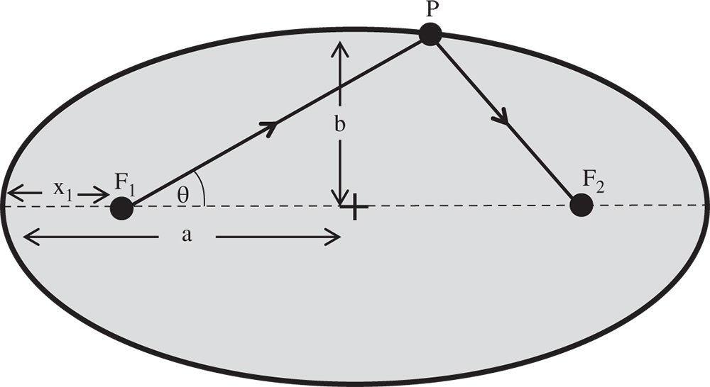
Figure 5.1 Ellipsoid of revolution.
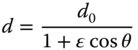
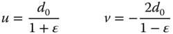
The parameter, ε, is the so-called eccentricity of the ellipse and is related to the conic parameter, k. In addition, the parameter, d0 is related to the base radius, R, as defined in the conic section formula in Eq. (5.1). The connection between the parameters is as set out in Eq. (5.3):

From the perspective of image formation, the two focal points, F1 and F2 represent the ideal object and image locations for this conic section. If x1 in Figure 5.1 represents the object distance u, i.e. the distance from the object to the nearest surface vertex, then it is also possible to calculate the distance, v, to the other focal point. These distances are presented below in the form of Eq. (5.2):
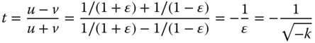
From the above, it is easy to calculate the conjugate parameter for this conjugate pair:
In fact, object and image conjugates are reversible, so the full solution for the conic constant is as in Eq. (5.5):
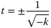
Thus, it is straightforward to demonstrate that for a conic section, there exists one pair of conjugates for which perfect image formation is possible. Of course, the most well known of these is where k = −1, which defines the paraboloidal shape. From Eq. (5.5), the corresponding conjugate parameter is −1 and relates to the infinite conjugate. This forms the basis of the paraboloidal mirror used widely (at the infinite conjugate) in reflecting telescopes and other imaging systems.
As for the spherical mirror, the effective focal length of the mirror remains the same as for the paraxial relationship:
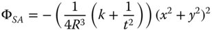
More generally, the spherical aberration produced by a conic mirror is of a similar form as for the spherical mirror but with an offset:
Worked Example 5.1 Simple Mirror-Based Magnifier
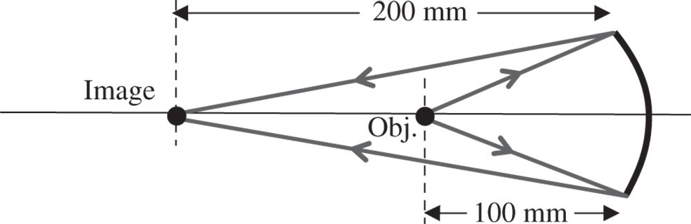
We wish to construct a simple magnification system with a simple conic mirror. The system magnification is to be two and the object distance 100 mm. There is to be no on axis aberration. What is the prescription of the mirror, i.e. base radius and conic constant?
It is assumed that object and image are located the same side of the mirror, so that, in this context, the image distance is −200 mm. The overall set up is illustrated in the diagram:
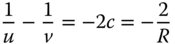
The base radius of the conic mirror is very simple to calculate as it follows the simple paraxial formula, as replicated in Eq. (5.6):
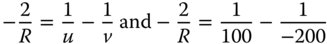
This gives R = −133 mm.
We now need to calculate the conjugate parameter, t:
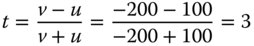
From Eq. (5.5) it is straightforward to see that k = −(1/t)2 and thus k = −0.1111. The shape is that of a slightly prolate ellipsoid.
The practical significance of a perfect on axis set up described in this example, is that it forms the basis of an ideal manufacturing test for such a conic surface. This will be described in more detail later in this text.
5.2.3 Conic Refracting Surfaces
There is no generic rule for conic refracting surfaces that generate perfect image formation for an arbitrary conjugate. However, there is a special condition for the infinite conjugate where perfect image formation results, as illustrated in Figure 5.2.
If the refractive index of the surface is n, assuming that the object is in air/vacuum, then the conic constant of the ideal surface is –n2. In fact, the shape is that of a hyperboloid. The abscissa of the hyperboloid effectively produce grazing incidence for rays originating from the object. By definition, therefore, the angle that the surface normal makes with the optical axis at the abscissa is equal to the critical angle. This restricts the maximum numerical aperture that can be collected by the system. With this constraint, it is clear that the maximum numerical aperture is equal to 1/n. In summary therefore:

Unfortunately, no other general condition for perfect image formation results for a conic surface. However, for perfect image correction, all orders of (on axis) aberration are corrected. Thus, although no condition for perfect image formation is possible, it is still possible, nevertheless, to correct for third order spherical aberration with a single refractive surface.
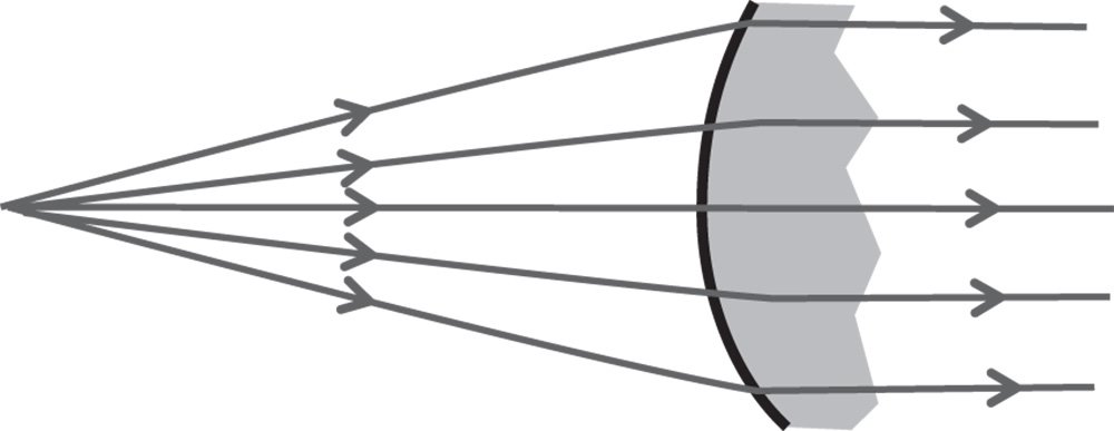
Figure 5.2 Single refractive surface at infinite conjugate.
5.2.4 Optical Design Using Aspheric Surfaces
The preceding discussion largely focused on perfect imaging in specific and restricted circumstances. However, even where perfect imaging is not theoretically possible, aspheric surfaces are extremely useful in the correction of system aberrations with a minimum number of surfaces. For more general design problems, therefore, even asphere terms may be added to the surface prescription. With the stop located at a specific surface, adding aspheric terms to the form of that surface can only control the spherical aberration at that surface. One perspective on the form of a surface is that second order terms only add to the power of that surface, whereas fourth order terms control the third order (in transverse aberration) aberrations. The reasoning behind this assertion may be viewed a little more clearly by expanding the sag of a conic surface in terms of even polynomial terms:

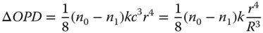
Adding a conic term to the surface, in addition to defining the curvature of the surface by its base radius, effectively adds an independent term to Eq. (5.9), effectively controlling two polynomial orders in Eq. (5.9). To this extent, adding separate additional second order and fourth order terms to the even asphere expansion in Eq. (5.1) is redundant. From the perspective of controlling third order aberrations, Eq. (5.9) confirms the utility of a conic surface in adding a controlled amount of fourth order optical path difference (OPD) to the system. In fact, the amount of OPD added to the system, to fourth order, is simply given by the change in sag produced by the conic surface multiplied by the difference in refractive indices. If the refractive index of the first medium is n0, and that of the second medium, n1, then the change in OPD produced by introducing a conic parameter of k is given by:
Equation (5.10) allows estimation of the spherical aberration produced by a conic surface introduced at the stop position. However, by virtue of the stop shift equations introduced in the previous chapter, providing fourth order sag terms at a surface remote from the stop not only influences spherical aberration, but also the other third order aberrations as well. In principle, therefore, by using aspheric surfaces, it is possible to eliminate all third order aberrations with fewer surfaces that would be possible with using just spherical surfaces alone. In fact, assuming that a system has been designed with zero Petzval curvature, it is only necessary to eliminate spherical aberration, coma, and astigmatism. Therefore, only three surfaces are strictly necessary. This represents a considerable improvement over a system employing only spherical surfaces. Notwithstanding the difficulties in manufacturing aspheric surfaces, some commercial camera systems are designed with this principal in mind.
Having introduced the underlying principles, it must be stated that design using aspheric surfaces is not especially amenable to analytical solution. In principle, of course, Eq. (5.10) could be used together with the relevant stop shift equations to compute analytically all third order aberrations. However, in practice, this is a rather cumbersome procedure and design of such systems proceeds largely by computer optimisation. Nevertheless, a clear understanding of the underlying principles is of invaluable help in the design process. An example, a simple two lens system, employing aspheric surfaces is sketched in Figure 5.3. This lens system replicates the performance of a three lens Cooke triplet with an aperture of f#5 and a field of view of 40°. Figure 5.3 is not intended to present a realistic and competitive design, but it merely illustrates the flexibility introduced by the incorporation of aspheric surfaces. In particular, it offers the potential to achieve the same performance with fewer surfaces.
Whilst aspheric components represent a significant enhancement to the toolkit of an optical designer, they represent something of a headache to the component manufacturer. As will be revealed later, in general, aspheric components are more difficult to manufacture and test and hence more costly. As such, their use is restricted to those situations where the advantage provided is especially salient. At the same time, advanced manufacturing techniques have facilitated the production of aspheric surfaces and their application in relatively commonplace designs, such as digital cameras, is becoming a little more widespread. Of course, the presence of conic and aspheric surfaces in large reflecting telescope designs is, by comparison, relatively well established.
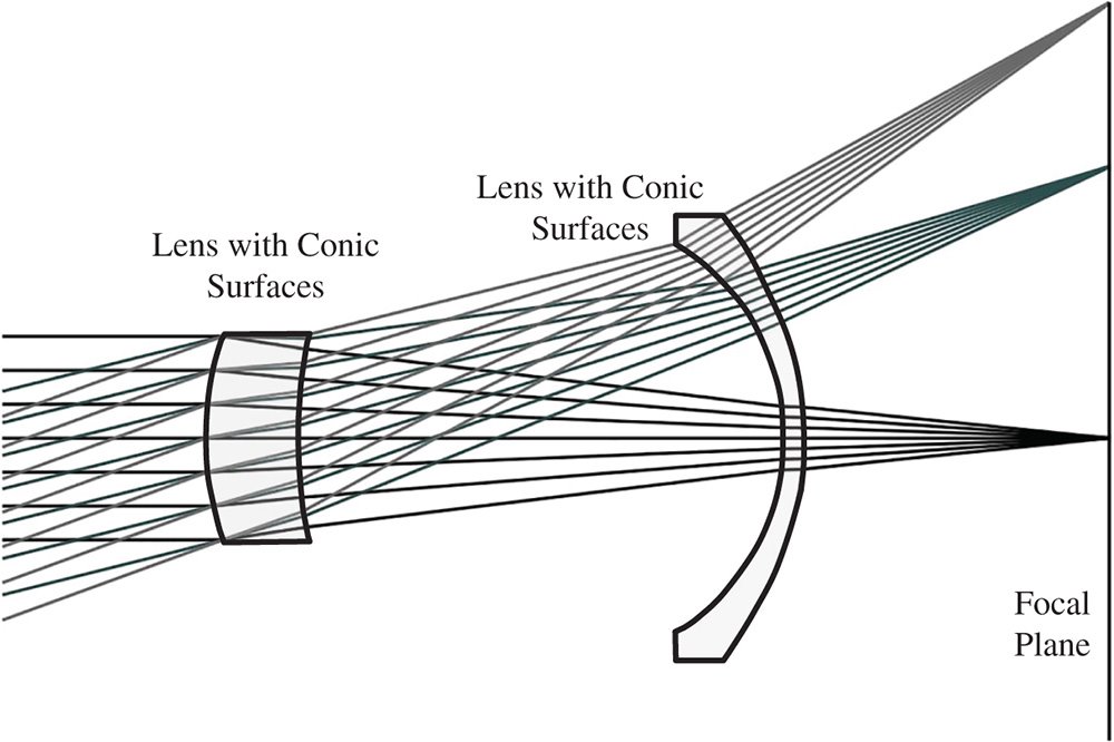
Figure 5.3 Simple two lens system employing aspheric components.
5.3 Zernike Polynomials
5.3.1 Introduction
In describing wavefront aberrations at any surface in a system, it is convenient to do so by expressing their value in terms of the two components of normalised pupil functions Px and Py. Where the magnitude of the pupil function is equal to unity, this describes the position of a ray at the edge of the pupil. With this description in mind, we now proceed to describe the normalised pupil position in terms of the polar co-ordinates, ρ and θ. This is illustrated in Figure 5.4.
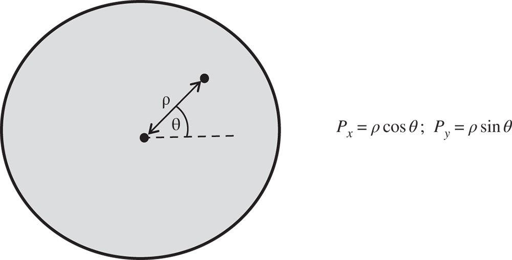
Figure 5.4 Polar pupil coordinates.
The wavefront error across the pupil can now be expressed in terms of ρ and θ. What we are seeking is a set of polynomials that is orthonormal across the circular pupil described. Any continuous function may be represented in terms of this set of polynomials as follows:

The individual polynomials are described by the term fi(ρ,θ), and their magnitude by the coefficient, Ai. The property of orthonormality is significant and may be represented in the following way:
The symbol, δij is the Kronecker delta. That is to say, when i and j are identical, i.e. the two polynomials in the integral are identical, then the integral is exactly one. Otherwise, if the two polynomials in the integral are different, then the integral is zero. The first property is that of normality, i.e. the polynomials have been normalised to one and the second is that of orthogonality, hence their designation as an orthonormal polynomial set.
Equations (5.11) and (5.12) give rise to a number of important properties of these polynomials. Initially we might be presented with a problem as to how to represent a known but arbitrary wavefront error, Φ(ρ,θ) in terms of the orthonormal series presented in Eq. (5.11). For example, this arbitrary wavefront error may have been computed as part of the design and analysis of a complex optical system. The question that remains is how to calculate the individual polynomial coefficients Ai. To calculate an individual term, one simply takes the cross integral of the function, Φ(ρ,θ), with respect to an individual polynomial, fi(ρ, θ):
By definition we have:
So, any coefficient may be determined from the integral presented in Eq. (5.13). The coefficients, Ai, clearly express, in some way, the magnitude of the contribution of each polynomial term to the general wavefront error. In fact, the magnitude of each component, Ai, represents the root mean square (rms) contribution of that component. More specifically, the total rms wavefront error is given by the square root of the sum of the squares of the individual coefficients. That this is so is clearly evident from the orthonormal property of the series:

5.3.2 Form of Zernike Polynomials
Following this general discussion about the useful properties of orthonormal functions, we can move on to a description of the Zernike circle polynomials themselves. They were initially investigated and described by Fritz Zernike in 1934 and are admirably suited to a solution space defined by a circular pupil. We will suppose initially, that the polynomial may be described by a component, R(ρ), that is dependent exclusively upon the normalised pupil radius and a component G(φ) that is dependent upon the polar angle, φ. That is to say:
We can make the further assumption that R(ρ) may be represented by a polynomial series in ρ. The form of G(φ) is easy to deduce. For physically realistic solutions, G(φ) must repeat identically every 2π radians. Therefore G(φ) must be represented by a periodic function of the form:
where m is an integer
This part of the Zernike polynomial clearly conforms to the desired form, since not only does it have the desired periodicity, but it also possesses the desired orthogonality. The parameter, m, represents the angular frequency of the polar dependence.
Having dealt with the polar part of the Zernike polynomial, we turn to the radial portion, R(ρ). The radial part of the Zernike polynomial, R(ρ), comprises of a series of polynomials in ρ. The form of these polynomials, R(ρ), depends upon the angular parameter, m, and the maximum radial order of the polynomial, n. Furthermore, considerations of symmetry dictate that the Zernike polynomials must either be wholly symmetric or anti-symmetric about the centre. That is to say, the operation r → −r is equivalent to φ → φ + π. For the Zernike polynomial to be equivalent for both (identical) transformations, for even values of m, only even polynomials terms can be accepted for R(ρ). Similarly, exclusively odd polynomial terms are associated with odd values of m.
Overall, the entirety of the set of Zernike polynomials are continuous and may be represented in powers of Px and Py or ρcos(φ) and ρsin(φ). It is not possible to construct trigonometric expressions of order, m, i.e. cos(mφ) and ρsin(mφ) where the order of the corresponding polynomial is less than m. Therefore, the polynomial, R(ρ), cannot contain terms in ρ that are of lower order than the angular parameter, m.
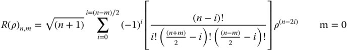
To describe each polynomial, R(ρ), it is customary to define it in terms of the maximum order of the polynomial, n, and the angular parameter, m. For all values of m (and n), the polynomial, R(ρ), may be expressed as per Eq. (5.17).
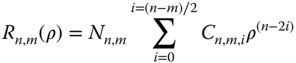
Cn,m,i represents the value of a specific coefficient
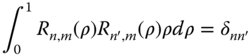
The parameter, Nn,m, is a normalisation factor. Of course, any arbitrary scaling factor may be applied to the coefficients, Cn,m,i, provided it is compensated by the normalisation factor. By convention, the base polynomial has a value of unity for ρ = 1. Of course, with this in mind, the purpose of the normalisation factor is to ensure that, in all cases, the rms value of the polynomial is normalised to one. It now remains only to calculate the values of the coefficients, Cn,m,i. These are determined from the condition of orthogonality which applies separately for Rn,m(ρ) and may be set out as follows:
The general formula for the coefficients Cn,m,i is set out in Eq. (5.18).
(5.19)
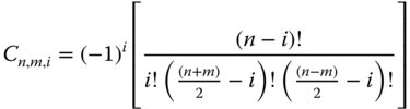
For i = n = 0, the value of the coefficient, Cn,m,i, as prescribed for the piston term, is unity. The value of the normalisation factor, Nn,m, is given in Eq. (5.20).

More completely we can express the entire polynomial:
The parameter, m, can take on positive or negative values as can be seen from Eq. (5.16). Of course, Eq. (5.16) gives the complex trigonometric form. However, by convention, negative values for the parameter m are ascribed to terms involving sin(mφ), whilst positive values are ascribed to terms involving cos(mφ).
Zernike polynomials are widely used in the analysis of optical system aberrations. Because of the fundamental nature of these polynomials, all the Gauss-Seidel wavefront aberrations clearly map onto specific Zernike polynomials. For example, spherical aberration has no polar angle dependence, but does have a fourth order dependence upon pupil function. This suggests that this aberration has a radial order, n, of 4 and a polar dependence, m, of zero. Similarly, coma has a radial order of 3 and a polar dependence of one. Table 5.2 provides a list of the first 28 Zernike polynomials.
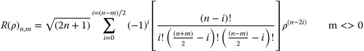
In Table 5.2, each Zernike polynomial has been assigned a unique number. This is the ‘Standard’ numbering convention adopted by the American National Standards Institute, (ANSI). It has the benefit of following the Born and Wolf notation logically, starting from the piston term which is denominated the zeroth term. If the ANSI number is represented as j, and the Born and Wolf indices as n, m, then the ANSI number may be derived as follows:
Unfortunately, a variety of different numbering conventions prevail, leading to significant confusion. This will be explored a little later in this chapter. As a consequence of this, the reader is advised to be cautious in applying any single digit numbering convention to Zernike polynomials. By contrast, the n, m numbering convention used by Born and Wolf is unambiguous and should be used where there is any possibility of confusion.
5.3.3 Zernike Polynomials and Aberration
As outlined previously, there is a strong connection between Zernike polynomials and primary aberrations when expressed in terms of wavefront error. Table 5.2 clearly shows the correspondence between the polynomials and the Gauss Seidel aberrations, with the 3rd order Gauss-Seidel aberrations, such as spherical aberration and coma clearly visible.
The power of the Zernike polynomials, as an orthonormal set, lies in their ability to represent any arbitrary wavefront aberration. Using the approach set out in Eq. (5.13), it is possible to compute the magnitude of any Zernike term by the cross integral of the relevant polynomial and the wavefront disturbance. Furthermore, the total root mean square (rms) wavefront error, as per Eq. (5.14), may be calculated from the RSS (root sum square) of the individual Zernike magnitudes. That is to say, the Zernike magnitude of each term represents its contribution to the rms wavefront error, as averaged over the whole pupil.
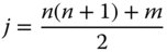
The use of defocus to compensate spherical aberration was explored in Chapters 3 and 4. In this instance, for a given amount of fourth order wavefront error, we sought to minimise the rms wavefront error by applying a small amount of defocus.
Hence, without defocus, adjustment, the raw spherical aberration produced in a system may be expressed as the sum of three Zernike terms, one spherical aberration, one defocus and one piston term. The total aberration for an uncompensated system is simply given by the RSS of the individual terms. However, for a compensated system only the Zernike n = 4, m = 0 term needs be considered. This then gives the following fundamental relationship: