The Unlucky Investor's Guide to Options Trading

Because delta is a measure of directional exposure, it plays a large role when hedging directional risks. For instance, if a trader currently has a 50Δ position on and wants the position to be relatively insensitive to directional moves in the underlying, the trader could offset that exposure with the addition of 50 negative deltas (e.g., two 25Δ long puts). The composite position is called delta neutral.

Gamma

is a second‐order Greek and a measure of the expected change in the option delta given a $1 change in the underlying price. Gamma is mathematically represented as follows:

(1.16)

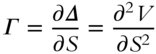
As with delta, the sign of gamma depends on the type of position:

● Long call and long put:

.

● Short call and short put:

.

In other words, if there is a $1 increase in the underlying price, then the delta for all long positions will become more positive, and the delta for all short positions will become more negative. This makes intuitive sense because a $1 increase in the underlying pushes long calls further ITM, increasing the directional exposure of the contract, and it pushes long puts further OTM, decreasing the inverse directional exposure of the contract and bringing the negative delta closer to zero. The magnitude of gamma is highest for ATM positions and lower for ITM and OTM positions, meaning that delta is most sensitive to underlying price movements at –50Δ and 50Δ .

Awareness of gamma is critical when trading options, particularly when aiming for specific directional exposure. The delta of a contract is typically transient, so the gamma of a position gives a better indication of the long‐term directional exposure. Suppose traders wanted to construct a delta neutral position by pairing a short call (negative delta) with a short put (positive delta), and they are considering using 20Δ or 40Δ contracts (all other parameters identical). The 40Δ contracts are much closer to ATM (50Δ ) and have more profit potential than the 20Δ positions, but they also have significantly more gamma risk and are less likely to remain delta neutral in the long term. The optimal choice would then depend on how much risk traders are willing to accept and their profit goals. For traders with high profit goals and a large enough account to handle the large P/L swings and loss potential of the trade, the 40Δ contracts are more suitable.

Theta

is a first‐order Greek that measures the expected P/L changes resulting from the decay of the option's extrinsic value (the difference between the current market price for the option and the intrinsic value of the option) per day. It is also commonly referred to as the time decay of the option. Theta is mathematically represented as follows:

(1.17)

where V is the price of the option (a call or a put) and t is time. The sign of theta depends on the type of position and is opposite gamma:

● Long call and long put:

.

● Short call and short put:

.

In other words, the time decay of the extrinsic value decreases the value of the long position and increases the value of the short position. For instance, a long call with a theta of –5 per one lot is expected to decline in value by $5 per day. This makes intuitive sense because the holders of the contract take gradual losses as their asset depreciates with time, a result of the value of the option converging to its intrinsic value as uncertainty dissipates. Because the extrinsic value of a contract decreases with time, the short side of the position profits with time and experiences positive time decay. The magnitude of theta is highest for ATM options and lower for ITM and OTM positions, all else constant.

There is a trade‐off between the gamma and theta of a position. For instance, a long call with the benefit of a large, positive gamma will also be subjected to a large amount of negative time decay. Consider these examples:

● Position 1: A 45 DTE, 16Δ call with a strike price of $50 is trading on a $45 underlying. The long position has a gamma of 5.4 and a theta of –1.3.

● Position 2: A 45 DTE, 44Δ call with a strike price of $50 is trading on a $49 underlying. The long position has a gamma of 7.9 and a theta of –2.2.

Compared to the first position, the second position has more gamma exposure, meaning that the contract delta (and the contract price) is more sensitive to changes in the underlying price and is more likely to move ITM. However, this position also comes with more theta decay, meaning that the extrinsic value also decreases more rapidly with time.

To conclude this discussion of the Black‐Scholes model and its risk measures, note that the outputs of all options pricing models should be taken with a grain of salt. Pricing models are founded on simplified assumptions of real financial markets. Those assumptions tend to become less representative in highly volatile market conditions when potential profits and losses become much larger. The assumptions and Greeks of the Black‐Scholes model can be used to form reasonable expectations around risk and return in most market conditions, but it's also important to supplement that framework with model‐free statistics.

Covariance and Correlation

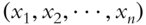
Up until now we have discussed trading with respect to a single position, but quantifying the relationships between multiple positions is equally important. Covariance quantifies how two signals move relative to their means with respect to one another. It is an effective way to measure the variability between two variables. For one signal, X, with observations

and mean

, and another, Y, with observations

and mean

the covariance between the two signals is given by the following:

(1.18)

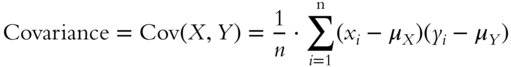
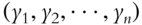
Represented in terms of random variables X and Y, this is equivalent to the following:15

(1.19)

Simplified, covariance quantifies the tendency of the linear relationship between two variables:

● A positive covariance indicates that the high values of one signal coincide with the high values of the other and likewise for the low values of each signal.

● A negative covariance indicates that the high values of one signal coincide with the low values of the other and vice versa.

● A covariance of zero indicates that no linear trend was observed between the two variables.

Covariance can be best understood with a graphical example. Consider the following ETFs with daily returns shown in the following figures: SPY (S&P 500), QQQ (Nasdaq 100), and GLD (Gold), TLT (20+ Year Treasury Bonds).

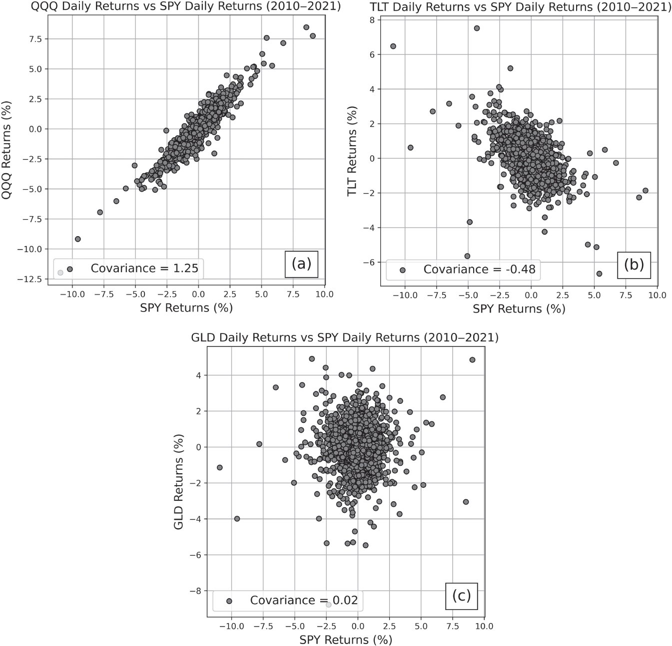
Figure 1.9 (a) QQQ returns versus SPY returns. The covariance between these assets is 1.25, indicating that these instruments tend to move similarly. (b) TLT returns versus SPY returns. The covariance between these assets is –0.48, indicating that they tend to move inversely of one another. (c) GLD returns versus SPY returns. The covariance between these assets is 0.02, indicating that there is not a strong linear relationship between these variables.

Covariance measures the direction of the linear relationship between two variables, but it does not give a clear notion of the strength of that relationship. Because the covariance between two variables is specific to the scale of those variables, the covariances between two sets of pairs are not comparable. Correlation, however, is a normalized covariance that indicates the direction and strength of the linear relationship, and it is also invariant to scale. For signals

with standard deviations

and covariance

, the correlation coefficient ρ (rho) is given by the following:

(1.20)

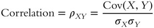
The correlation coefficient ranges from –1 to 1, with 1 corresponding to a perfect positive linear relationship, –1 corresponding to a perfect negative linear relationship, and 0 corresponding to no measured linear relationship. Revisiting the example pairs shown in Figure 1.9, the strength of the linear relationship in each case can now be evaluated and compared.

For Figure 1.9(a), QQQ returns versus SPY returns, the correlation between these assets is 0.88, indicating a strong, positive linear relationship. For Figure 1.9(b), TLT returns versus SPY returns, the correlation between these assets is –0.43, indicating a moderate, negative linear relationship. And for Figure 1.9(c), GLD returns versus SPY returns, the correlation between these assets is 0.00, indicating no measurable linear relationship between these variables. According to the correlation values for the pairs shown, the strongest linear relationship is between SPY and QQQ because the magnitude of the correlation coefficient is largest.

The correlation coefficient plays a huge role in portfolio construction, particularly from a risk management perspective. Correlation quantifies the relationship between the directional tendencies of two assets. If portfolio assets have highly correlated returns (either positively or negatively), the portfolio is highly exposed to directional risk. To understand how correlation impacts risk, consider the additive property of variance. For two random variables

with individual variances

and covariance

, the combined variance is given by the following:

(1.21)

When combining two assets, the overall impact on the uncertainty of the portfolio depends on the uncertainties of the individual assets as well as the covariance between them. Therefore, for every new position that occupies additional portfolio capital, the covariance will increase portfolio uncertainty (high correlation), have little effect on portfolio uncertainty (correlation near zero), or reduce portfolio uncertainty (negative correlation).

Конец ознакомительного фрагмента.

Текст предоставлен ООО «ЛитРес».

Прочитайте эту книгу целиком, купив полную легальную версию на ЛитРес.

Безопасно оплатить книгу можно банковской картой Visa, MasterCard, Maestro, со счета мобильного телефона, с платежного терминала, в салоне МТС или Связной, через PayPal, WebMoney, Яндекс.Деньги, QIWI Кошелек, бонусными картами или другим удобным Вам способом.

1

In liquid markets, which will be discussed in Chapter 5, American and European options are mathematically very similar.

2

The future value of the option should be used, but for simplicity, this approximates the future value as the current price of the option. The future value of the option premium is the current value of the option multiplied by the time‐adjusted interest rate factor.

3

Population calculations are used for all the moments introduced throughout this chapter.

4

This is the sum of the squared differences between each data point and the distribution mean, normalized by the number of data points in the set.

5

The skew of the returns distribution is also used to estimate the directional risk of an asset. The fourth moment (kurtosis) quantifies how heavy the tails of a returns distribution are and is commonly used to estimate the outlier risk of an asset.

6

Dividends can be accounted for in variants of the original model.

7

This application of Wiener processes as well as their use in financial mathematics are due to them arising as the scaling limit of simple random walk. A simple random walk is a discrete process that takes independent

steps with probability

. The scaling limit is reached by shrinking the size of the steps while speeding up their rate in such a way that the process neither sits at its initial location nor runs off to infinity immediately.

8

Note that, unless stated or shown otherwise, the date ranges throughout this book generally end on the first of the final year. For the range shown here, the data begins on January 1, 2010 and ends on January 1, 2015.

9

Displacement along the X‐axis is the difference between the current horizontal location of the particle and the previous horizontal location of the particle for each step.

10

Simple returns will also be approximated as normally distributed throughout this book. Although this is not explicitly implied by the Black‐Scholes model, it is a fair and intuitive approximation in most cases because the difference between log returns and simple returns is typically negligible on daily timescales.

11

d is a symbol used in calculus to represent a mathematical derivative. It equivalently represents an infinitesimal change in the variable it's applied to. dS(t) is merely a very small, incremental movement of the stock price at time t. ∂ is the partial derivative, which also represents a very small change in one variable with respect to variations in another.

12

The log function and log‐normal distribution are both covered in the appendix.

13

Order refers to the number of mathematical derivatives taken on the price of the option. Delta has a single derivative of V and is first‐order. Greeks of second‐order are reached by taking a derivative of first‐order Greeks.

14

In practice, the strike and underlying prices for 50Δ contracts tend to differ slightly due to strike skew.

15

The covariance of a variable with itself (e.g., Cov(X, X)) is merely the variance of the signal itself.